R notes

Programming in R (markdown and reproducibility)
- Quarto
Programming in R (installation and administration)
- Installing and updating R
- Managing R installations
Programming in R (software development)
Programming in R (language and evaluation)
Data munging
Statistics with R
Miscellaneous functions
RStudio
- Making it comfortable to work in
Further reading

Programming in R (markdown and reproducibility)

Quarto

.qmd files can be rendered to HTML or PDF from RStudio or the command line. To compile these from the command line use the following

quarto render <path/to/file.qmd>

The default settings during PDF generation are the following:

format:
pdf:
  documentclass: scrartcl
  papersize: letter

Code chunks

When loading libraries, you can avoid messages being printed with the following:

#| message: false

To include a table of contents, extend the preamble:

format:
  pdf:
    toc: true

Programming in R (installation and administration)

Installing and updating R

Last update was to 4.3.0 – Already Tomorrow

R updates frequently and things can break, so it is a good idea to keep your version of R reasonably up to date. You can obtain the source code for every version of R from CRAN. The steps involved in getting a particular version of R are as follows.

Ensure you have the necessary dependencies with sudo apt-get r-base.
Download the relevant source, e.g. R-4.2.1.tar.gz, and unzip it: tar -xvf R-X.Y.Z.tar.gz.
Run ./configure be sure to double check the output for configuration errors.
- If you are using this with RStudio, you will need to use --enable-R-shlib.
- If you are using SVG you may need to include --with-cairo.
- If you are using Wayland you might need --with-x=no.
- If you want extra optimisations add CFLAGS='-O3' CXXFLAGS='-O3' FFLAGS='-O3'
Run make and make info to compile R and the documentation.
- If you want to speed up compilation, make -j4 runs it in parallel across 4 coures.
Check that the compilation has worked properly with make check and address any issues that arise.
Install the executable with sudo make install and sudo make install-info.
Check it worked with R -e "sessionInfo()".
Profit!

Note that step 3 takes the longest, but this still took less than 20 minutes on my machine for R-4.1.0. After updating, you'll probably have lost all your packages, the following command can help with this.

my_pkgs <- c("ape",
             "argparse",
             "coda",
             "cowplot",
             "dplyr",
             "devtools",
             "deSolve",
             "future",
             "furrr",
             "ggplot2",
             "htmltools",
             "jsonlite",
             "phangorn",
             "purrr",
             "magrittr",
             "mcmc",
             "remotes",
             "reshape2",
             "stringr",
             "targets",
             "xml2")
install.packages(my_pkgs)

Last time when I updated the packages it said the default library was not writable so I used a personal library instead. Running the session with sudo fixed this. Old package versions hanging around can be found with .libPaths().

Notes

R.4.3.0 I needed to install xorg-dev prior to configuration to get this working with X.
R.4.2.3 I needed to use --with-x=no because I don't have X on the new laptop. Sadly, this seems to break plots. Also, make install put the binary in /usr/local/bin which appeared on the path after the location where the default installation is.
R.4.2.1
R.4.2.0 extends the pipe syntax, and some cases where if and while previously threw a warning now throw and error.
R-4.1.2
R-4.1.0 introduces some new syntax: |> for piping and some sugar for anonymous functions, eg \(x) x + 1 becomes function(x) x+1. After upgrading I could not create plots interactively, instead there was a message about unable to start device X11cairo. The fix for this was to set the DISPLAY environment variable to :1 where it was defaulting to :0.
R-4.0.4 Having some problems getting ggplot figures with transparency working but only in the PDF output. It hasn't been a problem so far so leaving it until next time. I was prompted to use a personal library for the packages this time, it is at /home/aez/R/x86_64-pc-linux-gnu-library/4.0.
R-4.0.2 needed me to install libpcre2-dev to get the configuration step to work. I also had to use sudo make install to install the executable where as previously it had not needed this level of permission. The update.packages command didn't work as expected this time, which prompted the installation list. I also needed to install a package build-dep before building this.

Managing R installations

There is an R package, rim, which manages installations: R installation manager.

Programming in R (software development)

Linting code

There is the stylr package for formating code. The following script makes it easy to format every R file in a directory from the command line.

#!/usr/bin/env Rscript
##
## Usage
## =====
##
## ./stylr.R <path_to_directory>
##
## Styles all the R files in the specified directory.
##
library(styler)


#' Style the R files in the specified directory
#'
#' @param dir_path The path to the directory containing the R files
#'
style_r_files <- function(dir_path) {
  if (!grepl("/$", dir_path)) {
    dir_path <- paste0(dir_path, "/")
  }

  files <- list.files(dir_path, pattern = "\\.R$", full.names = TRUE)
  lapply(files, style_file)

  if (length(files) > 0) {
    cat("Styled files:\n", paste(files, collapse = "\n"), "\n")
  } else {
    cat("No R files found in the specified directory.\n")
  }
}


main <- function() {
  args <- commandArgs(trailingOnly = TRUE)
  if (length(args) == 0) {
    stop("No directory specified. Usage: ./stylr.R <path_to_directory>", call. = FALSE)
  }

  style_r_files(args[1])
}

main()

Debugging

R makes it easy to shoot yourself in the foot, but it also makes it easy to patch your foot up again afterwards.

browser(): to create a breakpoint in your source code
=debugonce(): to enter the debugger next time you run a particular function.

Scripting with R

Running system commands with `base`

system2(command, args = character(),
        wait = TRUE,
        timeout = 0)

if wait is set to FALSE then this will run asynchronously
if timeout is set to a value greater than zero it will kill the process after that amount of time if it has not finished.

system2("ls", args = "/home/aez/Documents")

Running system commands with `processx`

There is the run command (from the library) which is a convenience function, otherwise you can use process$new(...) to create an instance of a new process.

Helper function for system commands

The following can be saved to a file and imported if you just need that one function.

message("loading the run_command function.")

#' Helper function for running system commands.
#'
#' Example
#' > run_command("stack build")
#' > run_command("Rscript R/make-simulation-configuration-1.R")
#'
run_command <- function(cmd, silent = TRUE, ...) {
  message(sprintf("\nRunning command:\n\t%s", cmd))
  tmp <- unlist(strsplit(cmd, " "))
  cmd_name <- head(tmp, 1)
  cmd_args <- tail(tmp, -1)
  std_val <- if (silent) {
    FALSE
  } else {
    ""
  }
  result <- system2(
    cmd_name,
    args = cmd_args,
    stdout = std_val,
    stderr = std_val,
    ...
  )
  if (result != 0) {
    stop(sprintf("command %s failed!", cmd))
  }
  return(NULL)
}

Working with files

In addition to the built-in functions described in this table, there is a package fs which aims to provide a consistent interface across operating systems and may be more appropriate if you are doing a lot of file manipulation.

Table 1: Some functions for working with filepaths.
Function	Use
`tempfile`	create temporary file
`basename`	get the file's name
`dirname`	get the file's directory
`file.exists`	predicate for file existance
`dir.exists`	predicate for directory existance

Error handling

Hadley has a nice description of how to handle these things in more detail, but here is a small example (from him)

show_condition <- function(code) {
  tryCatch(code,
    error = function(c) "error"
  )
}
show_condition(stop("!")) # evaluates to the string "error"
show_condition(10) # evalates to the numeric 10

R Packages by Wickham and Bryan

There is a new edition of the R packages book available online. Here are some notes about package creation based on reading through that book. R Packages tries to be friendly for those getting started and Writing R Extensions is the definitive reference.

Package development loop

library(devtools)
create_package("~/path/to/my/package") to set up the package
use_git()
use_r("funky") will set up an appropriate file for the named function. The standard is to use R/funky.R.
load_all() to bring the functions into the REPL to check it
use_mit_license("Alexander E. Zarebski")
Edit the DESCRIPTION
document()
check() to check the package works
install() to install on the current machine
Testing:
1. use_testthat()
2. use_test("funky") to template a test for the funky function
3. test() to run the tests
4. See these notes for details on how to write tests.
use_package("package_name") adds the named package as a dependency.
use_readme_rmd() sets up a README.
uninstall("<package>") to uninstall <package>

This information is also summarised in Section 1.20.

Package dependencies

The DESCRIPTION file is the place to go! Hadley says: add dependencies foo and bar with use_package("foo", "bar"). Use usethis::use_package as they have deprecated devtools::use_packag.

usethis::use_package("foo", "bar")

The DESCRIPTION will now have the following entry added

Imports:
    foo,
    bar

If the package depends on a specific version of the package this can be added too.

Imports:
    foo (>= 0.2),
    bar (>= 0.3.0.1)

Vignettes

Create a template vignette with usethis::use_vignette. There is an R Markdown Cheat Sheet

High performance computing

CRAN Task View for High Performance Computing

The package furrr provides purrr style functions which run in parallel. See the following snippet for an example

library(future)
plan(multiprocess)

y <- furrr::future_map(x, ~ f(.x))

WARNING It looks like furrr will kick up a fuss if f attempts to perform any IO. It's a good way to force the use of pure functions.

Packages I like

ape Analyses of Phylogenetics and Evolution

deSolve Solvers for Initial Value Problems of Differential Equations

lhs Latin Hypercube Samples

randomLHS(n,k) generates $n$ samples from $[0,1]^{k}$.

magrittr a forward pipe operator for R

There are many useful aliases exported by magrittr, the table below has some examples.

Alias	Function
`extract`	`[`
`extract2`	`[[`
`use_series`	`$`
`is_in`	`%in%`
`is_greater_than`	`>`
`set_colnames`	`colnames<-`

stringr Simple, Consistent Wrappers for Common String Operations

styler Non-Invasive Pretty Printing of R Code

testthat Unit Testing for R

truncnorm Truncated Normal Distribution

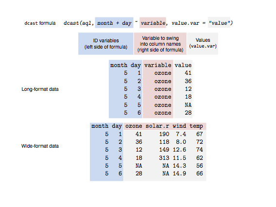
Reshaping dataframes with `reshape2`

Casting

Casting is difficult, this figure made by Sean C. Anderson helps

Command line arguments

The simplest example is probably what you'll need most of the time

## demo.R
args <- commandArgs(trailingOnly = TRUE)
print(args)

As an example consider the following command and output

$ Rscript demo.R 3 foo.csv
[1] "3"       "foo.csv"

Be careful when passing in numbers because they are read in as strings.

Command line arguments with `argparse`

See the vignette.

library(argparse)

# create parser object
parser <- ArgumentParser()

parser$add_argument(
         "-v",
         "--verbose",
         action = "store_true",
         default = FALSE,
         help = "Verbose output"
       )
parser$add_argument(
         "-s",
         "--seed",
         type = "integer",
         default = 1,
         help = "PRNG seed"
       )
parser$add_argument(
         "-p",
         "--parameters",
         type = "character",
         help = "Filepath to parameters JSON"
       )

args <- parser$parse_args()

Working with JSON

For parsing and encoding JSON there is the jsonlite package.

WARNING: by default jsonlite::write_json only uses 4 digits which is not enough for many scientific applications, unless there is a good reason not to, it is probably better to set digits = 16.

Examples

library(jsonlite)
read_json(<filepath>)
write_json(<object>, <filepath>, pretty = TRUE)

There are the toJSON and fromJSON functions but they are not needed most of the time.

Working with HTML

There is the htmltools package for generating HTML in R.

Example

library(htmltools)

my_html <-
  tags$html(
         tags$head(tags$title("My Title")),
         tags$body(
                tags$h1("Hello"),
                tags$div(
                       tags$h3("Hello World"),
                       tags$img(src = "the-world.png"),
                       tags$p("What a wonderful world!")
                     )
              )
       )

save_html(
  doRenderTags(my_html),
  file = "world.html"
)

produces the following HTML

<!DOCTYPE html>
<html lang="en">
<head>
<meta charset="utf-8"/>
<style>body{background-color:white;}</style>


</head>
<html>
  <head>
    <title>My Title</title>
  </head>
  <body>
    <h1>Hello</h1>
    <div>
      <h3>Hello World</h3>
      <img src="the-world.png"/>
      <p>What a wonderful world!</p>
    </div>
  </body>
</html>
</html>

Example: embedding PNG as string in HTML

The following function is useful if you want to avoid referencing external files in your HTML but still want to include figures.

#' An HTML tag encoding an image stored in a PNG.
#'
#' This uses the \code{base64enc} and \code{htmltools} packages.
#'
#' @param filepath is the path to the PNG
#' @param ... is additional arguments to \code{tags$img} such as style.
#'
png_as_img <- function(filepath, ...) {
  if (tools::file_ext(filepath) == "png") {
    b64 <- base64enc::base64encode(what = filepath)
    tags$img(
           src = paste("data:image/png;base64", b64, sep = ","),
           ...
         )
  } else {
    stop("Filepath given to png_as_img must be a PNG.")
  }
}

Example: including a table representation of a dataframe

#' An HTML tag encoding a data frame as a basic table.
#'
#' This uses the \code{xtable} package to generate the HTML for the table.
#'
#' @param df data.frame to create an table from
#' @param ... additional parameters for \code{xtable::xtable}.
#'
df_as_table <- function(df, ...) {
  tmp_file <- tempfile()
  print(xtable::xtable(df, ...),
        type = "html",
        file = tmp_file)
  return(tags$div(includeHTML(tmp_file)))
}

OUTDATED: Working with XML with `XML`

NOTE: It looks like xml2 might be a better choice for XML work, please see these notes instead.

Example I

The following snippet produces a file demo.xml

library(XML)

kappa_node <- xmlNode(
  "kappa",
  attrs = list(idref = "hky.kappa")
)

input_node <- xmlNode(
  "input",
  kappa_node,
  attrs = list(spec = "HKY", id = "hky")
)

z <- xmlNode(
  "beast",
  input_node,
  attrs = list(version = "2.0",
               namespace = "beast.core:beast.evolution.operators")
)

saveXML(
  z,
  file = "demo.xml",
  prefix = "<?xml version=\"1.0\" encoding=\"UTF-8\" standalone=\"no\"?>\n"
)

And here is the result

<?xml version="1.0" encoding="UTF-8" standalone="no"?>
<beast version="2.0" namespace="beast.core:beast.evolution.operators">
 <input spec="HKY" id="hky">
  <kappa idref="hky.kappa"/>
 </input>
</beast>

Example II

Given an XML file, demo.xml, we can read that into a list-like object:

library(XML)

xmlToList(xmlParse("demo.xml"))

Example III

We can read in the XML, edit one of the nodes by indexing into the object and replacing it, and then write it back to another file.

library(XML)

foo <- xmlTreeParse("demo.xml")$doc$children

bappa_node <- xmlNode(
  "bappa",
  attrs = list(idref = "hky.bappa")
)

foo[["beast"]][["input"]][["kappa"]] <- bappa_node

saveXML(
  foo$beast, # <-- need to specify the node.
  file = "demo-again.xml",
  prefix = "<?xml version=\"1.0\" encoding=\"UTF-8\" standalone=\"no\"?>\n"
)

Example IV

We can use XPath syntax to extract a particular node and then query its attributes.

foo <- xmlTreeParse("demo.xml")$doc$children$beast
kappa_node <- getNodeSet(foo, "//kappa[@idref='hky.kappa']")[[1]]
xmlGetAttr(kappa_node, "idref")

Working with Mustache templates

Example

library(whisker)

template <- readLines("./template.html")
data <- list( name = "Chris"
            , value = 10000
            , taxed_value = 10000 - (10000 * 0.4)
            , in_ca = TRUE
            )

writeLines(whisker.render(template, data), "./output.html")

where template.html might look like the following

Hello {{name}}
You have just won ${{value}}!
{{#in_ca}}
Well, ${{taxed_value}}, after taxes.
{{/in_ca}}

Unit testing with `testthat`

Here are the functions listed in Table 1 of the testthat paper by Hadley.

expect_true(x) # takes a logical.
expect_false(x)
expect_is(x, y)
expect_equal(x, y) # has a tolerance argument.
expect_equivalent(x, y)
expect_identical(x, y)
expect_matches(x, y)
expect_output(x, y)
expect_message(x, y)
expect_warning(x, y)
expect_error(x, y) # y is an regex for a error message.

Dependency management with `packrat`

Packrat is developed by the team at RStudio. It relies on the notion of a project, which we might think of as a single analysis or collection of related analyses. A project should live in a single directory.

Usage

To start a packrat project use

packrat::init()

This creates a directory packrat and a .Rprofile file. The profile file is how R knows to use the private library rather than the shared one. There is a file packrat/packrat.lock which contains the package details.

Packages are installed as usual with install.packages, but now they will be stored in the private packrat library. Packages are not added to the packrat.lock file until a snapshot of the current packages is made

packrat::snapshot()

If you want a status report from packrat about how the packages there is packrat::status. To install local packages, packrat needs to be told where they live

packrat::set_opts(local.repos = "<path/to/package>")

When moving a project between machines the installed packages will probably break. However, the packrat directory stores copies of the source for each of the packages so they can be restored.

packrat::restore()

Version control

The following files should be included into version control:

.gitignore can contain packrat/lib and packrat/src.
.Rprofile
packrat/packrat.opts
packrat/packrat.lock

The following explaination of the directory structure is given in the walkthrough

A packrat project contains a few extra files and directories. The init() function creates these files for you, if they don’t already exist.

packrat/packrat.lock: Lists the precise package versions that were used to satisfy dependencies, including dependencies of dependencies. (This file should never be edited by hand!)

packrat/packrat.opts: Project-specific packrat options. These can be queried and set with get_opts and set_opts; see ?"packrat-options" for more information.

packrat/lib/: Private package library for this project.

packrat/src/: Source packages of all the dependencies that packrat has been made aware of.

.Rprofile: Directs R to use the private package library (when it is started from the project directory).

Package and project management with `usethis`

Add dependencies to packages with usethis::use_package instead of devtools::use_package which is now deprecated. It is the same deal with use_vignette.

Date handling with `lubridate`

You may think you don't need to use this, but you are probably wrong. It won't take long before you need something that is painful to do in base date types, you may as well start out using this. It's part of the tidyverse, so it's safe.

Key data types for `lubridate`

An instant is an exact point in time,
an interval is the length of time between two instants,
a duration is the number of seconds between to instants,
a period is the length of time measured in units bigger than seconds (and hence only has a relative value).

String handling with `stringr`

Strings are another place where the built-in support is sufficient, but unpleasant to work with. The stringr package from the tidyverse makes this much easier and is organised to work well with the modern piping style.

function	use
`str_detect`	match like `grepl`, returning matches
`str_flatten`	flatten like `paste`
`str_interp`	string interpolation like `sprintf`
`str_replace`	substitution like `gsub`
`str_split`	split like `strsplit`
`str_subset`	filters strings like `grep`
`str_extract`	extracts pattern match
`str_to_lower`	converts to lower case

Documentation with `roxygen2`

R Packages: Function documentation

style	markup
italics	`\emph{}`
bold	`\strong{}`
mono-spaced	`\code{}`

Here is an example from R Packages:

#' Remove duplicated strings
#'
#' `str_unique()` removes duplicated values, with optional control over
#' how duplication is measured.
#'
#' @param string Input vector. Either a character vector, or something
#'  coercible to one.
#' @param ... Other options used to control matching behavior between duplicate
#'   strings. Passed on to [stringi::stri_opts_collator()].
#' @returns A character vector, usually shorter than `string`.
#' @seealso [unique()], [stringi::stri_unique()] which this function wraps.
#' @examples
#' str_unique(c("a", "b", "c", "b", "a"))
#'
#' @export
str_unique <- function(string, ...) {
  ...
}

For some mysterious reason, when you document a package and build a PDF of the manual it will include documentation for functions that you have not exported. There will be documentation for functions that are not made available to the user!

The solution appears to be to remove the corresponding .Rd files from man/ and then to build the manual from the remaining files. If you do not want to do this manually, the following script might help. WARNING: this assumes that you are only putting one function per file.

my_namespace <- readLines("NAMESPACE")
my_exported <- gsub(
  "export\\((.*)\\)",
  "\\1",
  grep("export", my_namespace, value = TRUE)
)

all_my_rd_files <-
  list.files("man", pattern = "\\.Rd$", full.names = TRUE)

not_exported_mask <-
  !gsub("man/(.*)\\.Rd", "\\1", all_my_rd_files) %in% my_exported
file.remove(all_my_rd_files[not_exported_mask])

Dates and times

as.Date is your friend.

Code	Value
`%d`	Day (integer)
`%m`	Month (integer)
`%b`	Abbreviated month (string)
`%B`	Month (string)
`%y`	Year (2 digits)
`%Y`	Year (4 digits)

`Rmath.h`

/*

  To compile and run this I used the following...


  $ sudo apt update
  $ sudo apt install r-mathlib
  $ sudo apt install r-base-dev
  $ gcc -o mathlibtest demo.c -lRmath -lm
  $ ./mathlibtest

 */

#include <stdio.h>

#define MATHLIB_STANDALONE 1
#include "Rmath.h"


int fib(int n) {
  if (n < 2) {
    return(1);
  } else {
    return(fib(n-1) + fib(n-2));
  }
}

int main(int ac, char** av)
{
  int n;
  double foo;

  for ( n = 0; n < 10; n = n + 1 ) {
    printf("%d\n", fib(n));
    foo = dnorm(1.0, 0.0, 1.0, 0);
    printf("%f\n", foo);
  }

  printf("hello, %s\n", "world");
  return 0;
}

Cheat sheets

Data structures

Hashmap

The environment builtin data structure can be used as a hashmap (since it hashes by default), a.k.a. map, dictionary, loopkup…

my_dict <- new.env(hash = TRUE)
my_dict[["key"]] <- 2
my_dict[["key"]] # will return 2.

Programming in R (language and evaluation)

Memory usage

To get the size of an object x in terms of its memory usage, run the following command:

print(format(object.size(x), units = "auto"))

You can get a print out of the current memory usage (and trigger a garbage collection) with the gc function. This can be helpful to call immediately after calling rm on large objects that are no longer needed.

Benchmarking and optimising impementations

This script demonstrates how to use the microbenchmark package in R to compare the performance of different implementations of the Fibonacci sequence. There are three different implementations of a function: fib_recursive, fib_iterative, and fib_memoised.

The script runs two sets of benchmarks:

mb_small: It runs each function 100 times on the input value of 20.
mb_large: Measures the performance of the iterative and memoized versions when computing the 150th Fibonacci number. The recursive version is not included because it would take an impractical amount of time to compute.

This demonstrates that the memoized version is faster than the iterative (_when evaluated multiple times_).

library(microbenchmark)

fib_true <- c(1,1,2,3,5,8,13)

fib_recursive <- function(n) {
  if (n <= 2) {
    return(1)
  } else {
    return(fib_recursive(n - 1) + fib_recursive(n - 2))
  }
}

fib_iterative <- function(n) {
  if (n <= 2) {
    return(1)
  }
  fib_values <- numeric(n)
  fib_values[1:2] <- 1
  for (i in 3:n) {
    fib_values[i] <- fib_values[i - 1] + fib_values[i - 2]
  }
  return(fib_values[n])
}


memoise <- function(f) {
  memo <- new.env(parent = emptyenv())
  function(n) {
    if (!exists(as.character(n), where = memo, inherits = FALSE)) {
      memo[[as.character(n)]] <- f(n)
    }
    memo[[as.character(n)]]
  }
}

fib_memoised <- memoise(function(n) {
  if (n <= 2) {
    return(1)
  } else {
    return(fib_memoised(n - 1) + fib_memoised(n - 2))
  }
})

stopifnot(all(sapply(X = 1:7, FUN = fib_recursive) == fib_true))
stopifnot(all(sapply(X = 1:7, FUN = fib_iterative) == fib_true))
stopifnot(all(sapply(X = 1:7, FUN = fib_memoised) == fib_true))

mb_small <- microbenchmark(
  fib_recursive(20),
  fib_iterative(20),
  fib_memoised(20),
  times = 100L
)
print(mb_small)

mb_large <- microbenchmark(
  fib_iterative(150),
  fib_memoised(150),
  times = 1000L
)
print(mb_large)

Functional programming support

library(magrittr)
library(purrr)

Here is a mapping between common functions in Haskell and their approximate analogue in R. These are mainly for use with lists of vectors.

Haskell	R (package)
`all`	`all`
`filter`	`keep` and `discard` (`purrr`)
`map`	`map` (`purrr`)
`scanl`	`accumulate` (`purrr`)

TODO Built-in functionality

|> pipes with _ for named arguments.

R/Haskell Prelude

## See https://hackage.haskell.org/package/base-4.15.0.0/docs/Prelude.html#v:dropWhile
drop_while <- function(p, xs) {
  if (length(xs) == 0) {
    xs
  } else {
    x <- head(xs, 1)
    remaining <- tail(xs, -1)
    if (p(x)) {
      drop_while(p, remaining)
    } else {
      remaining
    }
  }
}

## See https://hackage.haskell.org/package/base-4.15.0.0/docs/Prelude.html#v:takeWhile
take_while <- function(p, xs) {
  if (length(xs) == 0) {
    xs
  } else {
    x <- head(xs, 1)
    remaining <- tail(xs, -1)
    if (p(x)) {
      c(x, take_while(p, remaining))
    } else {
      c()
    }
  }
}

Program flow and control

Ternary operator

ifelse(test, yes, no)

Switch/case/which

This is similar to the match statement in Python.

centre <- function(x, type) {
  switch(type,
         mean = mean(x),
         median = median(x),
         trimmed = mean(x, trim = .1))
}

centre(rnorm(100), "mean")

Numbers

options(digits = 20) will cause the REPL to start printing 20 digits of the number.
ceiling floor and round behave as expected.
signif (significant figures) and round have a digits argument which can be used to specify the number of digits to use.

Metaprogramming and nonstandard evaluation

The following snippet demonstrates how to get the value of a variable given a string containing its symbol. There is a synonym as.name which derives from S terminology while "symbol" is LISP lingo.

a <- 1
eval(as.symbol("a"))

This doesn't seem to work unless you have string literals. Instead we can do the following

# this has a syntax error
data.frame(letters[1] = 2)

# this works!
eval(parse(text = sprintf("data.frame(%s = 2)", letters[1])))

Local aliases

The with function provides a way to define local variables based on a data frame or list, etc.

with(mtcars, mpg[cyl == 8  &  disp > 350])
# is the same as, but nicer than
mtcars$mpg[mtcars$cyl == 8  &  mtcars$disp > 350]

Object-oriented programming

S3

You can use the methods function which takes the name of a class as an argument to find a list of the methods available for that class.

R6 system

R6 classes are a popular way to bring traditional OOP to R, they have reference semantics.
R6 is available on CRAN
The R6Class function is used to declare classes, the (public) initialize function is used to create instances of this class with $new.
self is available within the class to describe the current object.
Assignment of fields is done with <- e.g., self$foo <- "bar"
Returning self invisibly (invisible(self)) makes methods chainable.
Active bindings are a way to carry out side effects when assigning values which has a syntax which looks like you are just assigning to a field.
Fields containing reference objects should be set in the initialize method unless you want the object to be shared across all instances of the class.
By default, objects get a clone method, which is shallow; deep cloning can be achieved by passing deep=TRUE.
There was a request for interfaces in R6, however Hadley suggested that this departed from the very minimalist goals of R6 so it will not be implemented.

Data munging

IO with R Data Serialisation (RDS)

RDS provides a simple (and very quick) way to save R objects to disk. This is a binary format and is computationally efficient, but is incompatible with other languages and not human readable, so there is a real trade-off there. It is very easy to use.

obj <- list(foo = "bar")

saveRDS(obj, "demo.rds")
new_obj <- readRDS("demo.rds")

Working with XML

The modern way for working with XML is via the xml2 package.

read_xml and write_xml for IO or start a new node from text.
xml_text (and xml_set_text) to get the text out of a node (and to modify it).
xml_set_attr to set attributes on a node. Note that if you want to set multiple attributes in a single command there is the function xml_set_attrs which takes a node and a named vector.
xml_add_child to add a child node to a parent.

Example I: creating a node and adding it to existing XML

Start with the following XML in demo.xml

<?xml version="1.0" encoding="UTF-8"?>
<bookstore>
    <book>
        <title lang="en">Harry Potter</title>
        <author>J K. Rowling</author>
        <year>2005</year>
        <price>29.99</price>
    </book>
</bookstore>

then run the following script

library(xml2)

bs <- read_xml("demo.xml")

new_book <- read_xml("<book><title/><author/><year/><price/></book>")

xml_set_attr(
  x = xml_find_first(new_book, "//title"),
  attr = "lang",
  value = "en")
xml_set_text(
  x = xml_find_first(new_book, "//title"),
  value = "Nineteen Eighty-Four"
)
xml_set_text(
  x = xml_find_first(new_book, "//author"),
  value = "G Orwell"
)
xml_set_text(
  x = xml_find_first(new_book, "//year"),
  value = "1949"
)
xml_set_text(
  x = xml_find_first(new_book, "//price"),
  value = "8.99"
)

xml_add_child(bs, new_book)
write_xml(bs, "demo2.xml")

to get the new file demo2.xml

<?xml version="1.0" encoding="UTF-8"?>
<bookstore>
  <book>
    <title lang="en">Harry Potter</title>
    <author>J K. Rowling</author>
    <year>2005</year>
    <price>29.99</price>
  </book>
  <book>
    <title lang="en">Nineteen Eighty-Four</title>
    <author>G Orwell</author>
    <year>1949</year>
    <price>8.99</price>
  </book>
</bookstore>

Example II: swapping a node for a new one in existing XML

Starting with demo2.xml from the previous example

<?xml version="1.0" encoding="UTF-8"?>
<bookstore>
  <book>
    <title lang="en">Harry Potter</title>
    <author>J K. Rowling</author>
    <year>2005</year>
    <price>29.99</price>
  </book>
  <book>
    <title lang="en">Nineteen Eighty-Four</title>
    <author>G Orwell</author>
    <year>1949</year>
    <price>8.99</price>
  </book>
</bookstore>

we can use the script

library(xml2)

bs <- read_xml("demo2.xml")

new_cd <- read_xml("<cd><title/><artist/><year/></cd>")

xml_set_text(
  x = xml_find_first(new_cd, "//title"),
  value = "Lateralus"
)
xml_set_text(
  x = xml_find_first(new_cd, "//artist"),
  value = "Tool"
)
xml_set_text(
  x = xml_find_first(new_cd, "//year"),
  value = "2001"
)

old_book <- xml_find_first(bs, "//book[title='Harry Potter']")
xml_replace(old_book, new_cd)
write_xml(bs, "demo3.xml")

which produces demo3.xml shown below

<?xml version="1.0" encoding="UTF-8"?>
<bookstore>
  <cd>
    <title>Lateralus</title>
    <artist>Tool</artist>
    <year>2001</year>
  </cd>
  <book>
    <title lang="en">Nineteen Eighty-Four</title>
    <author>G Orwell</author>
    <year>1949</year>
    <price>8.99</price>
  </book>
</bookstore>

Example III: A helpful function for getting and setting attributes

The functions in this snippet allows you to look up a node with XPath syntax and then read one of the attributes or set its value. There is an optional argument in the former to get the value returned as a numeric.

#' Find the first matching node and return the named attribute
#'
#' @param x the XML document
#' @param xp the xpath
#' @param the attribute
#' @param as_numeric boolean for casting to numeric (default is FALSE)
#'
xml_find_attr <- function(x, xp, attr, as_numeric=FALSE) {
  a <- xml_attr(xml_find_first(x, xpath = xp), attr)
  if (!as_numeric) {
    a
  } else {
    as.numeric(a)
  }
}

#' Find the first matching node and set the named attribute
#'
#' @param x the XML document
#' @param xp the xpath
#' @param attr the attribute
#' @param v the value for the attribute
#'
xml_find_set_attr <- function(x, xp, attr, v) {
  n <- xml_find_first(x, xpath = xp)
  xml_set_attr(n, attr, v)
}

Example IV: linting/formatting/beautifying XML

If you have the js-beautify node package installed, the following function will lint a file in place.

#' Format an XML file in place using js-beautify
#'
#' @param x is the filepath
#'
beautify_xml <- function(x) {
  system2(command = "html-beautify", args = c("-f", x, "-r"))
}

Joins

There are several ways to join data frames using dplyr, the folling snippet demonstrates a full join which duplicates records where necessary and will fill in missing values. Although the data in the joined data frame does not depend on the order of the arguments, the ordering of the rows does.

foo <- data.frame(x = 1:3, y = letters[1:3])
bar <- data.frame(x = c(2:4,2:4), z = LETTERS[1:6])
dplyr::full_join(foo,bar)

Joining, by = "x"
  x    y    z
1 1    a <NA>
2 2    b    A
3 2    b    D
4 3    c    B
5 3    c    E
6 4 <NA>    C
7 4 <NA>    F

Aggregation

aggregate(formula = Petal.Length ~ Species, FUN = mean, data = iris)

is equivalent to

library(dplyr)
iris %>%
  group_by(Species) %>%
  summarise(mean_petal_length = mean(Petal.Length))

Selecting columns

See starts_with and ends_with, and matches which takes strings to describe columns.

Sorting rows

Base R approach

iris[order(iris$Sepal.Length),]

Tidyverse approach

You can use the following command to generate a figure that shows the rows of iris are certainly not sorted by the length, although they are sorted by species.

plot(iris$Sepal.Length, col = iris$Species)

The dplyr::arrange function will sort the rows of a data frame based on a selected column, respecting groupings if the data are grouped. The following demonstrates how this works.

tmp1 <- iris |>
  dplyr::group_by(Species) |>
  dplyr::arrange(Sepal.Length, .by_group = TRUE) |>
  as.data.frame()

plot(tmp1$Sepal.Length, col = tmp1$Species)

Note that if you forget to group in this way it will just sort all of the rows!

tmp2 <- iris |>
  dplyr::arrange(Sepal.Length) |>
  as.data.frame()

plot(tmp2$Sepal.Length, col = tmp2$Species)

Renaming columns

If you want to programmatically rename the columns of a data frame the dplyr::rename_with function takes a function .fn from strings to strings defining a renaming rule. The columns that this get applied to are selected with the argument to the .cols argument.

Statistics with R

GLM

Here is an example of fitting a negative binomial GLM using the MASS package.

Linear regression `lm`

NOTES

Zero-inflated regression

The following snippet demonstrates how to perform a zero-inflated Poisson regression.

library(pscl)
library(boot)
set.seed(1)

n <- 1000
x1 <- rnorm(n = n)
x2 <- rnorm(n = n)
z1 <- rnorm(n = n)
z2 <- rnorm(n = n)
true_prob_zinf <- inv.logit(2 * z1 + 0 * z2)
zero_inflation <- rbernoulli(n = n,
                             p = true_prob_zinf)

true_count_means <- exp(2 * x1 - 1 * x2 + 1)
maybe_count <- rpois(n = n,
                     lambda = true_count_means)

y <- ifelse(zero_inflation, 0, maybe_count)

df <- data.frame(y = y,
                 x1 = x1,
                 x2 = x2,
                 z1 = z1,
                 z2 = z2)

my_zinb <- zeroinfl(formula = y ~ x1 + x2 | z1 + z2,
                    data = df, dist = "poisson")

true_mean <- true_prob_zinf * 0 + (1 - true_prob_zinf) * true_count_means

plot(log(true_mean), log(fitted(my_zinb)))
abline(0,1)

TODO Mathematical optimisation

nlm

Computational geography and cartography

See my other notes on this.

Differential equations with `deSolve`

Basic SIR example

Simple SIR model

\[ \frac{ds}{dt} = -\beta s i \quad\text{and}\quad \frac{di}{dt} = \beta s i - \gamma i. \]

The following demonstrates how to solve this system with deSolve.

library(deSolve)

sir_diff <- function(time, state, params) {
    with(as.list(c(params, state)), {
        ds <- - beta * susceptible * infectious
        di <- beta * susceptible * infectious - gamma * infectious
        list(c(ds, di))
    })
}

params <- c(beta = 1.2, gamma = 1)
state <- c(susceptible = 0.99, infectious = 0.01)
times <- seq(from = 0, to = 20, length = 100)
pd <- matrix(nrow = 2, ncol = 2, data = 0)
out1 <- deSolve::ode(state, times, sir_diff, parms = params)

SIR example with C implementation

Then we can implement the differential in C as

/* file sirmod.c */
#include <R.h>

static double params[2];
#define beta params[0]
#define gamma params[1]

/* initializer */
void initmod(void (* odeparams)(int *, double *))
{
  int N=2;
  odeparams(&N, params);
}

/* Derivatives and 1 output variable */
void derivs (int *neq, double *t, double *y, double *ydot,
             double *yout, int *ip)
{
  if (ip[0] <1) error("nout should be at least 1");
  ydot[0] = -beta*y[0]*y[1];
  ydot[1] = beta*y[0]*y[1] - gamma*y[1];
  yout[0] = 1.0-y[0]+y[1];
}
/* END file sirmod.c */

Then we need to compile this and load the object for use of deSovle

system("R CMD SHLIB sirmod.c")
dyn.load("sirmod.so")
out2 <- deSolve::ode(state, times, func = "derivs", parms = params,
                     dllname = "sirmod", initfunc = "initmod", nout = 1,
                     outnames = "recovered")

MCMC (without `Stan`)

There is the package mcmc which looks like it does a solid job of the basics, although it takes an opinionated stance on how this should be done. Be careful with how you interpret the batch arguments. The interface is designed for testing out tuning parameters to find something that works; make the most of this design.

coda is probably what you want to use to check the output beyond basic diagnostic plots.

Thinning (destructive)

This snippet demonstrates how to subset a data frame. It is a destructive change, but since MCMC samples can be large you may not want the additional cost of creating a copy.

demo_df <- data.frame(x = 1:100, y = rnorm(100))

## take every third sample
thinning_factor <- 3

demo_df <- demo_df[seq(from = 1, to = nrow(demo_df), by = thinning_factor), ]

(Nonparametric) density estimation with `KernSmooth`

Here is an example looking at how to use KernSmooth.

library(KernSmooth)

set.seed(1)

x <- c(rpois(n = 500, lambda=10),
       rpois(n = 500, lambda = 30))

f_x <- function(x, ...) {
  0.5 * (dpois(x = x, lambda = 10, ...) +
         dpois(x = x, lambda = 30, ...))
}

x_mesh <- 0:100
y_mesh <- f_x(x_mesh)


kde_obj <- bkde(x, bandwidth = 3, range.x = c(0,100), gridsize = 101)

r_kde_samples <- sample(x = kde_obj$x,
                       size = length(x),
                       replace = TRUE,
                       prob = pmax(0, kde_obj$y))

type_char <- c("true", "estimate")

density_df <- data.frame(x = c(x_mesh, x_mesh),
                         y = c(y_mesh, pmax(0, kde_obj$y)),
                         type = rep(type_char, each = 101))

sample_df <- data.frame(x = c(x, r_kde_samples),
                        type = rep(type_char,
                                   each = length(x)))

ggplot() +
  geom_histogram(data = sample_df,
                 mapping = aes(x = x, y = ..density.., fill = type),
                 bins = 25,
                 size = 3,
                 position = "dodge") +
  geom_line(data = density_df,
            mapping = aes(x = x, y = y, colour = type))

Miscellaneous functions

Function to save a ggplot to both PNG and SVG

#' Save a ggplot to both PNG and SVG.
#'
#' @param filepath is the path to save the plot to.
#' @param plot is the ggplot object to save.
#' @param ... are additional arguments to pass to ggsave.
#'
#' @examples
#' ggsave_plus("plot.png", ggplot() + geom_point(aes(x = 1:10, y = 1:10))
#'
ggsave_plus <- function(filepath, plot, ...) {
  if (stringr::str_ends(filepath, ".png")) {
    filepath_png <- filepath
    filepath_svg <- str_replace(filepath, ".png", ".svg")
  } else if (stringr::str_ends(filepath, ".svg")) {
    filepath_svg <- filepath
    filepath_png <- str_replace(filepath, ".svg", ".png")
  }

  ggplot2::ggsave(plot, filename = filepath_png, ...)
  ggplot2::ggsave(plot, filename = filepath_svg, ...)
}

Quantile functions of truncated distributions

The truncnorm package provides a clean way to work with normal distributions that have been truncated to a finite range of values. I wanted the analogous function for the quantile function of the log-normal distribution but this wasn't in the package. Here is an implementation and a basic test of such a quantile function.

.qtruncnorm <- function(p, a = -Inf, b = Inf, mean = 0, sd = 1) {
  ut_cdf_a <- pnorm(a, mean = mean, sd = sd)
  ut_cdf_b <- pnorm(b, mean = mean, sd = sd)
  ut_p <- pnorm(a, mean = mean, sd = sd) + p * (pnorm(b, mean = mean, sd = sd) - pnorm(a, mean = mean, sd = sd))
  return(qnorm(ut_p, mean = mean, sd = sd))
}


.test_ps <- runif(1000)
stopifnot(
  max(abs(.qtruncnorm(.test_ps, a = -1, b = 2, mean = 3) - truncnorm::qtruncnorm(.test_ps, a = -1, b = 2, mean = 3))) < 1e-13
)


.qtrunclnorm <- function(p, a = -Inf, b = Inf, meanlog = 0, sdlog = 1) {
  ut_cdf_a <- plnorm(a, meanlog = meanlog, sdlog = sdlog)
  ut_cdf_b <- plnorm(b, meanlog = meanlog, sdlog = sdlog)
  ut_p <- plnorm(a, meanlog = meanlog, sdlog = sdlog) + p * (plnorm(b, meanlog = meanlog, sdlog = sdlog) - plnorm(a, meanlog = meanlog, sdlog = sdlog))
  return(qlnorm(ut_p, meanlog = meanlog, sdlog = sdlog))
}


.test_ps <- seq(from = 0.2, to = 0.9, length = 10)
stopifnot(
  max(abs(.qtrunclnorm(.test_ps, a = 0, b = 10^5, meanlog = 3) - qlnorm(.test_ps, meanlog = 3))) < 1e-14
)
.test_ps <- runif(1000)
stopifnot(
  !(max(abs(.qtrunclnorm(.test_ps, a = 0, b = 10^3, meanlog = 3) - qlnorm(.test_ps, meanlog = 3))) < 1e-14)
)
stopifnot(
  (max(abs(.qtrunclnorm(.test_ps, a = 0, b = 10^5, meanlog = 3) - qlnorm(.test_ps, meanlog = 3))) < 1e-14)
)

Read BEAST2 log file

See the example in the notes here.

Generating LaTeX summary of GLM

We can use the xtable package to generate a table in LaTeX that displays a sensible summary of estimates. The following function streamlines this process a little bit.

#' Convert GLM Fit to LaTeX-Ready xtable
#'
#' This function takes a GLM fit object, formats the summary information,
#' and returns an xtable object for LaTeX export.
#'
#' @param fit A GLM fit object obtained through the `glm()` function.
#' @param num_fmt A string indicating the format for numerical values (default is "%f").
#' @param ... Additional arguments passed to xtable.
#'
#' @return An xtable object containing formatted GLM summary data.
#'
#' @examples
#' fit <- glm(mpg ~ wt + hp, data=mtcars, family=gaussian())
#' tab <- glm_fit_as_xtable(fit, num_fmt="%.2f")
#' print.xtable(tab, include.rownames=FALSE, type="latex", file="demo-latex-table.tex")
#'
#' @importFrom xtable xtable
#' @importFrom stats as.data.frame confint summary
#'
glm_fit_as_xtable <- function(fit, num_fmt="%f", ...) {

  ns <- c(var = "Variable",
          est_and_ci = "Estimate and CI (95%)",
          sig = "Significance",
          p_val = "Pr(>|t|)")

  fs_df <- as.data.frame(summary(fit)$coefficient)[, c(1,4)]

  tmp <- confint(fit)

  fs_df[[ns['var']]] <- rownames(fs_df)
  est_and_ci_fmt <-
    sprintf("%s (%s, %s)", num_fmt, num_fmt, num_fmt)
  fs_df[[ns['est_and_ci']]] <-
    sprintf(est_and_ci_fmt, fs_df$Estimate, tmp[,1], tmp[,2])
  fs_df[[ns['sig']]] <-
    ifelse(fs_df[[ns['p_val']]] < 0.05 , "*", "")

  rownames(fs_df) <- NULL

  # Return xtable object
  return(xtable(fs_df[ns[c(1,2,3)]],
                align = c("l", "l", "r", "c"),
                ...))
}

This will return an xtable object which still needs to be printed in a slightly strange way, the following example might help.

library(xtable)

fit <- glm(mpg ~ wt + hp, data=mtcars, family=gaussian())

print.xtable(glm_fit_as_xtable(fit, num_fmt="%.2f"),
             include.rownames = FALSE,
             type = "latex",
             file = "demo-latex-table.tex")

Mini test suite

If you ever wanted to run tests in a script without needing another package, here is a little function that you can use to do this. It is configured with the global variable RUN_TESTS.

RUN_TESTS <- TRUE

## Define a little tester function that evaluates an expression and
## stops with a suitable error message if it evaluates to false
tts_test <- function(expr) {
  if (RUN_TESTS) {
    if (!expr) {
      cat("Test expression: ", deparse(substitute(expr)), "\n")
      stop("Test failed")
    } else {
      message("Test passed")
    }
  } else {
    return(invisible())
  }
}

Step function

Step function construction

The following snippet defines a vectorised step function.

#' Return a vectorized step function.
#'
#' This function creates a vectorized step function that changes
#' values at specified time points (`ts`). The resulting step function
#' will produce a constant value between each pair of consecutive
#' times in `ts`, and return the corresponding value in `vs` for any
#' given input. If an input value is less than the first time in `ts`,
#' it will return the first value in `vs`. If an input value is
#' greater than or equal to the last time in `ts`, it will return the
#' last value in `vs`.
#'
#' @param ts A numeric vector of times at which the step function
#'   changes values. Must be sorted in strictly increasing order and
#'   have at least one element.
#' @param vs A numeric vector of values corresponding to the steps.
#'   Must have one more element than `ts` because the function needs
#'   to cover all time ranges, including values less than the first
#'   time and values greater than or equal to the last time.
#'
step_function_factory <- function(ts, vs) {
  n <- length(ts)
  if (n < 1) {
    stop("need at least one step time.")
  }
  if (all(sort(ts, decreasing = FALSE) != ts)) {
    stop("times must be sorted in strictly increasing order.")
  }
  if (length(vs) != (1 + n)) {
    stop("if there are n step times there must be n+1 values.")
  }

  step_func <- function(x) {
    m <- length(x)
    y <- numeric(m)
    mask <- logical(m)
    mask <- x < ts[1]
    y[mask] <- vs[1]
    if (n > 1) {
      for (ix in seq.int(2, n)) {
        mask <- (ts[ix-1] <= x) & (x < ts[ix])
        y[mask] <- vs[ix]
      }
    }
    mask <- x >= ts[n]
    y[mask] <- vs[n+1]
    return(y)
  }

  return(
    list(
      func = step_func,
      times = ts,
      values = vs
    )
  )
}

Here is a demonstration of it in action producing Figure 1

t1s <- c(2.0, 3.0)
v1s <- c(3.0, 2.5, 3.5)
demo1 <- step_function_factory(t1s, v1s)
t2s <- c(1.0)
v2s <- c(1.0, 2.0)
demo2 <- step_function_factory(t2s, v2s)

x <- seq(from = 0, to = 4, length = 200)
y1 <- demo1$func(x)
y2 <- demo2$func(x)

png('step-function-demo.png',
    width = 1.618 * 300,
    height = 300,
    units = "px")
plot(x, y1, 'l', col = 'black', ylab = "", ylim = c(0.5, 3.5))
lines(x, y2, col = 'black')
points(t1s, demo1$func(t1s), col = 'blue', cex = 3, pch = 16)
points(t1s, demo1$func(t1s - 1e-10), col = 'red', cex = 3, pch = 1)
points(t2s, demo2$func(t2s), col = 'blue', cex = 3, pch = 16)
points(t2s, demo2$func(t2s - 1e-10), col = 'red', cex = 3, pch = 1)
dev.off()

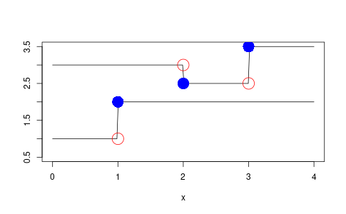
Figure 1: Example of step function result.

Applying binary functions to step functions

The class of step functions is closed under the point-wise application of binary functions. What? This means if you have two functions $f(x)$ and $g(x)$ which are step functions, then $h(x) := f(x) + g(x) $ is also a step function, and more generally $h^{F}(x) := F(f(x), g(x))$ is a step function given some binary function $F$. This can be implemented as follows

#' Return a vectorised step function resulting from the point-wise application
#' of a binary function to two step functions.
#'
#' @param step_func_a a step function (see \code{step_function_factory}.)
#' @param step_func_b a step function (see \code{step_function_factory}.)
#' @param binary_func a binary function.
#'
map_step_function <- function(step_func_a, step_func_b, binary_func) {
  times_c <- sort(union(step_func_a$times, step_func_b$times))
  n <- length(times_c)
  values_c <- numeric(n + 1)
  values_c[1] <- binary_func(
    step_func_a$func(step_func_a$times[1] - 1),
    step_func_b$func(step_func_b$times[1] - 1)
  )
  for (ix in seq.int(n)) {
    values_c[ix+1] <- binary_func(
      step_func_a$func(times_c[ix]),
      step_func_b$func(times_c[ix])
    )
  }
  return(step_function_factory(times_c, values_c))
}

Here is a demonstration of it in action producing Figure 2

demo3 <- map_step_function(demo1, demo2, function(x, y) { x / y })
y3 <- demo3$func(x)
t3s <- c(t2s, t1s)

png('step-function-binary-demo.png',
    width = 1.618 * 300,
    height = 300,
    units = "px")
plot(x, y3, 'l', col = 'black', ylab = "")
points(t3s, demo3$func(t3s), col = 'blue', cex = 3, pch = 16)
points(t3s, demo3$func(t3s - 1e-10), col = 'red', cex = 3, pch = 1)
dev.off()

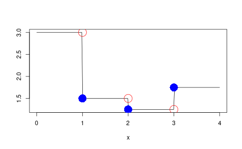
Figure 2: The result of combining two step functions.

And here is another example in which we use date-time objects for the times of the step functions. The resulting figure is shown in Figure 3.

library(lubridate)

ts1 <- ymd_hms(c("2024-01-01 00:00:00",
                 "2024-01-02 00:00:00",
                 "2024-01-03 00:00:00"))
vs1 <- c(10, 30, 20, 40)
step_func_a <- step_function_factory(ts1, vs1)

ts2 <- ymd_hms(c("2024-01-02 00:00:00",
                 "2024-01-03 00:00:00",
                 "2024-01-04 00:00:00"))
vs2 <- c(15, 25, 35, 45)
step_func_b <- step_function_factory(ts2, vs2)

step_func_c <- map_step_function(step_func_a,
                                 step_func_b,
                                 function(x, y) { x + y })

times_to_evaluate <- seq(from = ymd_hms("2023-12-31 00:00:00"),
                         to = ymd_hms("2024-01-05 00:00:00"),
                         length = 100)
result <- step_func_c$func(times_to_evaluate)

png('step-function-dates-demo.png',
    width = 1.618 * 300,
    height = 300,
    units = "px")
plot(times_to_evaluate, result, 'l', col = 'black', ylab = "", ylim = c(0, 90))
lines(times_to_evaluate, step_func_a$func(times_to_evaluate), col = 'blue')
lines(times_to_evaluate, step_func_b$func(times_to_evaluate), col = 'red')
dev.off()

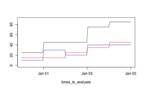
Figure 3: An example using dates as time

A multivariate generalisation of the step function

The multi version of the step function returns a vector of values when evaluated at a single point and a matrix when given a vector of times.

#' Return a vectorized step vector-function.
#'
#' This is similar to the `step_function_factory` function except that
#' it returns a vector-value instead of a single value. The use case
#' for this is to be able to have a distribution of step functions
#' obtained from a posterior sample.
#'
#' @param ts A numeric vector of times at which the step function
#'   changes values. Must be sorted in strictly increasing order and
#'   have at least one element.
#' @param vs_list A list of numeric vectors of values corresponding to
#'   the steps. Each vector must have one more element than `ts`
#'   because the function needs to cover all time ranges, including
#'   values less than the first time and values greater than or equal
#'   to the last time.
#'
step_function_factory_multi <- function(ts, vs_list) {
  n <- length(ts)
  if (n < 1) {
    stop("need at least one step time.")
  }
  if (all(sort(ts, decreasing = FALSE) != ts)) {
    stop("times must be sorted in strictly increasing order.")
  }
  if (length(vs_list) != (1 + n)) {
    stop("if there are n step times there must be n+1 values.")
  }
  vec_length <- length(vs_list[[1]])
  if (!all(sapply(vs_list, function(x) length(x) == vec_length))) {
    stop("all vectors in the list must be the same length.")
  }

  step_func <- function(x) {
    m <- length(x)
    y <- matrix(numeric(m * vec_length), nrow = m)
    mask <- logical(m)
    mask <- x < ts[1]
    y[mask, ] <-  t(replicate(sum(mask), vs_list[[1]]))
    if (n > 1) {
      for (ix in seq.int(2, n)) {
        mask <- (ts[ix - 1] <= x) & (x < ts[ix])
        y[mask, ] <- t(replicate(sum(mask), vs_list[[ix]]))
      }
    }
    mask <- x >= ts[n]
    y[mask, ] <- t(replicate(sum(mask), vs_list[[n + 1]]))
    return(y)
  }

  return(
    list(
      func = step_func,
      times = ts,
      values = vs_list
    )
  )
}

And here is an example of how to use this.

t4s <- c(2.0, 3.0)
num_funcs <- 5
v4s <- list(rnorm(num_funcs, sd = 0.2, mean = 1),
            rnorm(num_funcs, sd = 0.2, mean = 3),
            rnorm(num_funcs, sd = 0.2, mean = 2))
vals_range <- v4s |> unlist() |> range()
demo4 <- step_function_factory_multi(t4s, v4s)

x <- seq(from = 0, to = 4, length = 200)
y <- demo4$func(x)

Which produces the following Figure 4.

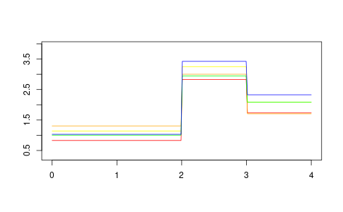
Figure 4: An example using multivariate values

cols <- c('red', 'orange', 'yellow', 'green', 'blue')
png('step-function-multi-demo.png',
    width = 1.618 * 300,
    height = 300,
    units = "px")
plot(x, y[,1], 'l', col = cols[1], ylim = vals_range + c(-0.5, 0.5), ylab = "", xlab = "")
for (ix in 2:num_funcs) {
  lines(x, y[,ix], col = cols[ix])
}
dev.off()

Number of lines in a file

The num_lines_in_file function returns the number of lines in a file which is useful to help guard against attempting to parse an empty file with read.csv.

num_lines_in_file <- function(fp) {
  wc_stdout <- system2(command = "wc", args = c("-l", fp), stdout = TRUE)
  as.numeric(head(unlist(strsplit(x = wc_stdout, split = " ")),1))
}

Julian day of the year

#' Julian day of the year
#'
#' > j_day("2014-01-03", "2014-01-01")
#' 3
j_day <- function(date_string, first_day_of_year_string) {
  as.integer(as.Date(date_string) - as.Date(first_day_of_year_string)) + 1
}

RStudio

Making it comfortable to work in

Open the preferences menu: Tools then Global Options.
In the Code menu enable Vim bindings (obviously).
In the Appearance menu, make the font and theme comfortable for your eyes.
In Pane Layout ensure the console and source panes dominate the screen.
Keep in mind the following (default) keybindings:
- Alt+Shift+K shows the keybinding cheatsheet
- Crtl+1 focuses on source
- Ctrl+2 focuses on the console
- Crtl+Enter runs the selected lines
The Tools menu has a tool for modifying keybindings

R notes

Table of Contents

Programming in R (markdown and reproducibility)

Quarto

Code chunks

Table of contents

Programming in R (installation and administration)

Installing and updating R

Notes

Managing R installations

Programming in R (software development)

Linting code

Debugging

Scripting with R

Running system commands with base

Running system commands with processx

Helper function for system commands

Working with files

Error handling

R Packages by Wickham and Bryan

Package development loop

Package dependencies

Vignettes

High performance computing

Packages I like

ape Analyses of Phylogenetics and Evolution

deSolve Solvers for Initial Value Problems of Differential Equations

lhs Latin Hypercube Samples

magrittr a forward pipe operator for R

stringr Simple, Consistent Wrappers for Common String Operations

styler Non-Invasive Pretty Printing of R Code

testthat Unit Testing for R

truncnorm Truncated Normal Distribution

Reshaping dataframes with reshape2

Casting

Command line arguments

Command line arguments with argparse

Working with JSON

Examples

Working with HTML

Example

Example: embedding PNG as string in HTML

Example: including a table representation of a dataframe

OUTDATED: Working with XML with XML

Example I

Example II

Example III

Example IV

Working with Mustache templates

Example

Unit testing with testthat

Dependency management with packrat

Usage

Version control

Package and project management with usethis

Date handling with lubridate

Key data types for lubridate

String handling with stringr

Documentation with roxygen2

Dates and times

Rmath.h

Cheat sheets

Data structures

Hashmap

Programming in R (language and evaluation)

Recommended reading

Memory usage

Benchmarking and optimising impementations

Functional programming support

TODO Built-in functionality

R/Haskell Prelude

Program flow and control

Ternary operator

Switch/case/which

Numbers

Metaprogramming and nonstandard evaluation

Local aliases

Object-oriented programming

S3

R6 system

Running system commands with `base`

Running system commands with `processx`

Reshaping dataframes with `reshape2`

Command line arguments with `argparse`

OUTDATED: Working with XML with `XML`

Unit testing with `testthat`

Dependency management with `packrat`

Package and project management with `usethis`

Date handling with `lubridate`

Key data types for `lubridate`

String handling with `stringr`

Documentation with `roxygen2`

`Rmath.h`

Linear regression `lm`

Differential equations with `deSolve`

MCMC (without `Stan`)

(Nonparametric) density estimation with `KernSmooth`