beast2-aez-notes

Home

Links
Notes
Simulating data
- MASTER
Tools and useful R functions
Examples

Notes

Understanding BEAUti

The configuration of BEAUti is done using template files. There are a couple of blog posts intended to make it easier to write these files:
- Better BEAUti Templates
- Debugging BEAUti Templates

Build a BEAST2

Clone the BEAST2 repository.
- git clone git@github.com:CompEvol/beast2.git
Build the project by running ant.
- If you don't care about running the tests ant compile-all does the compilation without running the tests.
Run the desired program:
- java -cp build/dist/beast.jar beast.app.beauti.Beauti
- java -cp build/dist/beast.jar beast.app.beastapp.BeastMain

Note that you can clock on the little '?' in Beauti to get the location that packages are stored at.

Notes

v2.6.7:

TODO Understanding Packages

Bouckaert has a blog post about building package from source from mid-2021. The following line from the Babel build.xml (which is the example package used in the blog post)

<property name="beast2path" location="../beast2" />

makes it sound like it assumes that BEAST2 will be in the same directory as the packages during compilation.

Installing packages from source

Remco has written about building and installing packages from source.

The key steps include the following:

Get the package.zip files, e.g., BEASTlabs.v2.0.2.zip
Find the ~/.beast/2.X/ directory and make sure there is an empty subdirectory with the same name as the package, e.g., ~/.beast/2.X/BEASTlabs should be empty.
Use zip -o <path/to/package.zip> from within the directory to install the package.

TODO Configuring IntelliJ for writing a package

There are notes on Java and IntelliJ here. I have no idea if this is the correct way that BEAST2 packages should be set up, but this has worked for me in the past, and provided there are a sufficient number of unit tests I assume it should work…

Note that the build.xml probably assumes that BEAST2 and your code are in sibling directories.
Build the BEAST2 project first and then close it and open your project (probably based on the results of ant skeleton).
Click through File – Project Settings – Modules – <YOUR/PACKAGE> and then using the + (add) button, tell IntelliJ that you want to add a Module Dependency, which will be BEAST2.
When building the package, if it complains about missing packages, you may need to add JAR files in the same way.

Understanding BEAST2

A class diagram showing the relationship between the various classes that are relevant to tree priors are shown in Figure 2.
The BEASTInterface is an interface which all BEAST-objects must implement, the BEASTObject class implements that interface and most objects we care about will derive from BEASTObject.
The StateNode is akin to the stochastic node of H\"{o}hna et al (2014), ie it is a random variable. State nodes can be changed by operators.
The CalculationNode is akin to the deterministic node of H\"{o}hna et al (2014), ie it is a deterministic function of its input.
See Figure 1 which is helpful for understanding where state and calculations nodes sit in this formulation.
The TreeDistribution (which extends the Distribution abstract class) is the foundation for both the classes deriving from SpeciesTreeDistribution (which are the birth-death models) and various coalescent models.
There is a ModelBuilder application for visualising a computation.
Operator s are used to change the value of StateNode (of which RealParameter is an example).

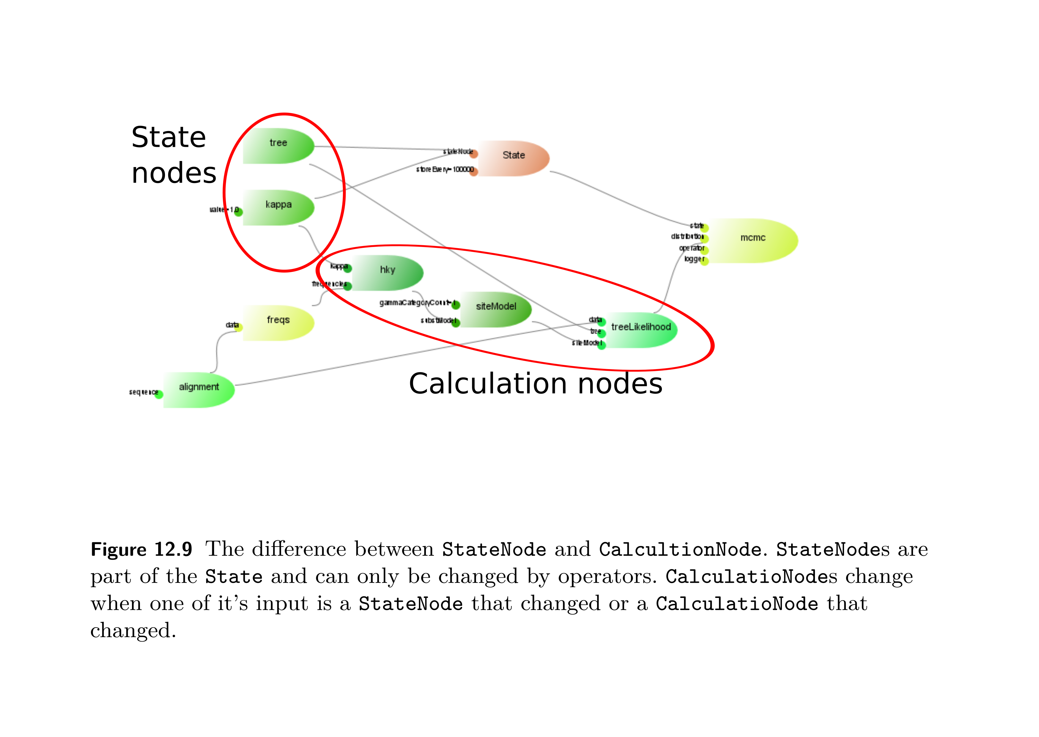
Figure 1: Figure from Drummond and Bouckaert (2015).

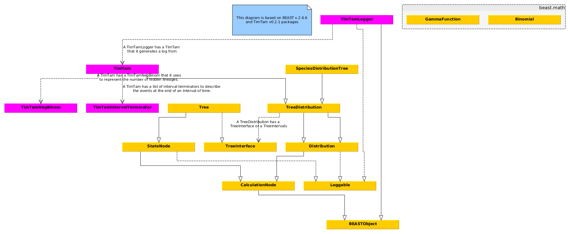
Figure 2: Class diagram relating to tree priors in BEASTv2.6

In Fig 3 we see API of a Tree.

Figure 3: Class diagram relating to the tree in BEASTv2.7

Figure 4: Class diagram relating to the MCMC in BEASTv2.7

Packages provided by BEAST2

Inference

The beast.inference.distribution package (which previously was part of either the beast.core or beast.math packages) contains the classes from the Apache Commons Mathematics Library, (it appears to use version 2.x). Since the triangular distribution was not added until 3.0 it is not part of BEAST2.

Understanding `bdsky`

To understand the implementation of time varying parameters see the following:

Skyline (interface)
SkylineSegement (class)
SimpleSkyline (class)
MultiSkyline (class)

To understand how this implements the BDSky model see the following:

BDSSkylineSegment (class)
BDSParameterization (abstract class)
CanonicalParameterization (class)
R0Parameterization (class)

which all culminates in ParameterizedBirthDeathSkylineModel (class) which is the class that actually does the main calculation.

Skyline (interface)
```
public interface Skyline { }
```
Skyline is an interface provided by the bdsky package
- This represents a multivariate right continuous function on a domain \([a,\infty)\).
- The interface requires the methods getSegments, getValue, getValues, getTimes and getDimension.
- Things that implement Skyline look like lists of
SkylineSegment (class)
```
public class SkylineSegment { }
```
SkylineSegment is a class provided by the bdsky package
- This represents an interval of time, \([a,b)\), and a vector of values assigned to that time.
- There are methods start and end to get the start, \(a\), and end, \(b\) times of the interval.
SimpleSkyline (class)
```
public class SimpleSkyline extends CalculationNode implements Skyline { }
```
SimpleSkyline is a class provided by the bdsky package which represents a piece-wise constant function (with a one dimensional range).
MultiSkyline (class)
```
public class MultiSkyline extends CalculationNode implements Skyline { }
```
MultiSkyline is a class provided by the bdsky package which is really just a wrapper around a list of =SimpleSkyline=s, which takes care of splitting up time into the required number of segments.
BDSSkylineSegment (class)
```
public class BDSSkylineSegment extends SkylineSegment { }
```
BDSSkylineSegment is a class that wraps the SkylineSegment and specialises it for use as the parameterisation of the BDS model. Both the CanonicalParameterization and the R0Parameterization make use of this class, constructing their skyline segments with it.
BDSParameterization (abstract class)
```
public abstract class BDSParameterization extends CalculationNode { }
```
BDSParameterization is an abstract class provided by the bdsky package which provides a template for writing classes which provide novel parameterisations of the model. The CanonicalParamterization and R0Parameterization are two classes that inherit from this.
CanonicalParameterization (class)
```
public class CanonicalParameterization extends BDSParameterization { }
```
CanonicalParameterization is a class provided by the bdsky package which extends (ie inherits from) the BDSParameterization abstract class and represents the parameterisation in terms of the birth rate, death rate, sampling rate, and removal probability (which is important for sampled ancestors).
R0Parameterization (class)
```
public class R0Parameterization extends BDSParameterization { }
```
R0Parameterization is a class provided by the bdsky package which extends (ie inherits from) the BDSParameterization abstract class and represents the parameterisation in terms of the reproductive number, total becoming uninfectious rate, the sampling proportion and the removal probability upon sampling.
ParameterizedBirthDeathSkylineModel (class)
```
public class ParameterizedBirthDeathSkylineModel extends SpeciesTreeDistribution { }
```
ParameterizedBirthDeathSkylineModel is a class provided by the bdsky package which does the actual calculation, ie it has a calculateTreeLogLikelihood method.

Understanding the XML

Chapter 13 of (, ) focuses on how BEAST uses XML to specify a computation.

There are some reserved attributes (this table) and element names (this table) that BEAST attributes special meaning to.
The namespace attribute of the beast element specifies where classes are looked for. The comma-separated list is searched in order, but you can use the full name in cases where there could be a name-clash.
The input can be replaced with the name to simplify the specification.

Table 1: Reserved attributes
Attribute name	Purpose
`id`	Unique identifier
`idref`	Reference to another element
`name`	The part of the parent it plugs into
`spec`	The Java class to use

Table 2: Reserved tags
Tag name	Associated BEAST-object
`run`	`beast.core.Runnable`
`distribution`	`beast.core.Distribution`
`operator`	`beast.core.Operator`
`logger`	`beast.core.Logger`
`data`	`beast.evolution.alignment.Alignment`
`sequence`	`beast.evolution.alignment.Sequence`
`state`	`beast.core.State`
`parameter`	`beast.core.parameter.RealParameter`
`tree`	`beast.evolution.tree.Tree`
`input`	reserved name
`map`	macro to simplify `spec`
`plate`	for-loop style macro

The plate macro

The XML

<plate var="n" range="v1,v2,v3" >
    <parameter id="value.$(n)" a="foo" b="$(n)" />
</plate>

becomes

<parameter id="value.v1" a="foo" b="v1" />
<parameter id="value.v2" a="foo" b="v2" />
<parameter id="value.v3" a="foo" b="v3" />

Understanding the MCMC application

Occasionally, BEAST will dump the state of the chain to a file: for example, running demo.xml will typically store the state in another file called demo.xml.state. This state file allows you to resume a sampler at a later date if you want to continue the chain. The following will demonstrate how to do this.

Grab a BEAST2 XML, we will use demo.xml. We can then run this as follows:

java -cp <path/to/beast.jar> beast.app.beastapp.BeastMain -seed 1 demo.xml

In addition to the log file, this should also produce a file demo.xml.state. We can rename this file to whatever we want, for example mv demo.xml.state burnt.xml.state. Then we can restart the sampler at the point saved in that file:

java -cp <path/to/beast.jar> beast.app.beastapp.BeastMain -seed 1 -resume -statefile burnt.xml.state demo.xml

The flag -resume tells BEAST to append to the end of the existing log file and -statefile burnt.xml.state specifies which file to read the state from (otherwise it will look for one called demo.xml.state).

Starting tree

Navigating tree space can be difficult so it is useful to be able to start a chain off on a sensible tree. There is a tab in BEAUti (which is hidden by default) that allows you to define the starting tree, or a distribution to sample it from. You can make this tab visible via the View menu. In the Starting tree tab you can choose a distribution to sample a tree from, a clustering algorithm to generate a tree, or you can specify the tree manually in Newick format.

When specifying the tree via Newick, the following snippets demonstrate how this is done for BEAST2.6 and BEAST2.7:

<!-- 2.6 -->
<init spec='beast.util.TreeParser' id='NewickTree.t:XYZ26'
initial="@Tree.t:XYZ26" taxa='@XYZ26' IsLabelledNewick="true"
newick="((your,(tree,goes)),here)"/>

<!-- 2.7 -->
<init spec='beast.base.evolution.tree.TreeParser' id='NewickTree.t:XYZ26'
initial="@Tree.t:XYZ26" taxa='@XYZ26' IsLabelledNewick="true"
newick="((your,(tree,goes)),here)"/>

Priors

The ExcludablePrior class from the BEASTLabs package provides a way to set a prior distribution on an individual element of a RealParameter. This can be used with the ScaleOperator when you need a way to change just some parts of a real vector.

To make use of this class you will need to have BEASTLabs installed. The following snippet demonstrates how to use it. It considers a length three real parameter and applies a beta prior to the second element, as indicated by the xInclude attribute.

<map name="excludablePrior" >beast.math.distributions.ExcludablePrior</map>

<excludablePrior id="PRIOR-ID" name="distribution" x="PARAM-ID-REF" xInclude="false true false">
  <Beta name="distr">
    <parameter spec="parameter.RealParameter" estimate="false" name="alpha">2.0</parameter>
    <parameter spec="parameter.RealParameter" estimate="false" name="beta">2.0</parameter>
  </Beta>
</excludablePrior>

Operators

The ScaleOperator has an input indicator which can be used to select elements of a RealParameter to scale. Frustratingly, there is not the same functionality for the random walk operators (or any other operator for that matter). If you want to set a particular parameter element to a particular value while allowing the others to change, this might be what you need.

To use this, you need to construct a Boolean parameter vector. You could do this by creating one in the state node as a stateNode and then referencing it in the operator.

Tuning operators

Not all operators will auto-tune. If there are integer parameters you may need to do some small example runs to get a sensible rate of mixing. Some things online say you should aim for approximately \(30\%\) acceptance of samples.

Simulating data

MASTER

Piece-wise constant rates

The Reaction page on the MASTER Wiki describes how to use time varying rates.

Tools and useful R functions

You can run both beast and beauti from the command line as they are both available in the beast.jar. In the case of beauti it will be something like java -sp <path/to/beast.jar> beast.app.beauti.Beauti.
Tracer, FigTree, TempEst and TreeAnnotator all comes as a separate jar files. You can just click on the jar file and it should run the program correctly.
- My TempEst notes

Cogsworth

The cogsworth ANT file is intended to simplify some of the typical tasks involved in running BEAST2 from the command line. You can get a copy here!

Web beautify

Having a linter for XML is helpful. The tool js-beautify seems decent: LINK and GitHub. You can configure this if you do not like the default style it uses. Just add the following as .jsbeautifyrc in the root of your project.

{
    "indent_size": 4,
    "preserve_newlines": true,
    "wrap_attributes": "force-aligned"
}

The following function handles calling the beautifier from within R

#' Run js-beautify on the given file.
#'
#' @param x is the path to the XML file.
#'
beautify_xml <- function(x) {
  system2(command = "html-beautify", args = c("-f", x, "-r"))
}

Read BEAST2 log file

The following function reads a log file into a suitable dataframe.

#' Read a BEAST2 log file into a data frame.
#'
#' @param filename is the path to the log file.
#' @param burn is the number to remove from the start.
#' @param take_last is the number to take from the end.
#'
#' @return data frame containing the samples.
#'
read_beast2_log <- function(filename, burn=0, take_last=NA) {
  y <- read.csv(filename, sep = "\t", comment.char = "#")
  if (is.na(take_last) && burn >= 0) {
    return(tail(y, nrow(y) - burn))
  } else if (!is.na(take_last) && burn == 0) {
    return(tail(y, take_last))
  } else {
    stop("Unsupported arguments given to read_beast2_log.")
  }
}

Pretty printing Tracer output

The following little script can be used to translate a summary produced by Tracer into something that is easier to use in documents.

#!/usr/bin/env Rscript
# -*- mode:ess-mode; -*-
#'
#' tracer-table
#' ============
#'
#' Tool to convert tracer summary to an org-mode/markdown style table.
#'
#' Usage
#' -----
#'
#' ./tracer-table --input <demo.txt> --output demo.org
#'

suppressPackageStartupMessages(library(argparse))

parser <- ArgumentParser()

parser$add_argument(
         "-v",
         "--verbose",
         action = "store_true",
         default = FALSE,
         help = "Verbose output"
       )
parser$add_argument(
         "-i",
         "--input",
         type = "character",
         help = "Input file"
       )
parser$add_argument(
         "-o",
         "--output",
         type = "character",
         help = "Output file"
       )

args <- parser$parse_args()


main <- function(args) {
  foo <- readLines(args$input) |>
    gsub(pattern = "\t", replacement = " | ") |>
    gsub(pattern = "^", replacement = "| ") |>
    gsub(pattern = "$", replacement = " |")
  tbl_header <- head(foo, 1)
  tbl_hline <- tbl_header |>
    gsub(pattern = "[_\ a-zA-Z]", replacement = "-") |>
    gsub(pattern = "-\\|-", replacement = "-+-")
  tbl_body <- tail(foo, -1)
  bar <- c(tbl_header, tbl_hline, tbl_body)
  writeLines(text = bar, con = args$output)
}

if (!interactive()) {
  args <- parser$parse_args()
  main(args)
}

BEAST2 as an MCMC engine: part I

This example looks at how to use BEAST2 to simulate from a standard normal distribution using MCMC. The XML for this has the following structure

<?xml version="1.0" encoding="UTF-8" standalone="no"?>
<beast version="2.0">

  <<targetDistribution>>

  <<mcmc>>

</beast>

The targetDistribution specifies the distribution we will sample from and the mcmc specifies how details of the MCMC algorithm.

The target distribution

We use a Prior to represent the distribution because this makes it easy to evaluate the distribution at a particular value.

<!-- targetDistribution -->
<distribution id="posterior" spec="beast.base.inference.distribution.Prior" x="@x">
  <distr spec="beast.base.inference.distribution.Normal" mean="0.0" sigma="1.0" />
</distribution>

MCMC

We use a run tag to specify the MCMC. This requires a state object to describe the parameters we are sampling, the distribution over the state, and an operator and logger to perturb the state and record the results.

<!-- mcmc -->
<run chainLength="10000000" id="mcmc" preBurnin="100" spec="beast.base.inference.MCMC">

    <state id="state" storeEvery="1000">
        <parameter estimate="true" id="x" name="stateNode" value="1.0" />
    </state>

    <distribution idref="posterior" />

    <operator spec="beast.base.inference.operator.RealRandomWalkOperator"
              windowSize="0.1"
              useGaussian="true"
              weight="1.0"
              parameter="@x" />

    <logger id="screenlog" logEvery="1000000">
        <log idref="x" />
    </logger>

    <logger fileName="beast.csv"
            id="tracelog"
            logEvery="10000"
            model="@posterior">
        <log idref="posterior" />
        <log idref="x" />
    </logger>

</run>

Running the sampler

Here is the command to actually run this program.

java -jar beast.jar -seed 1 -overwrite example-01.xml

I have used the -overwrite flag because otherwise it will prompt you each time unless you change the output file name.

Visualising the results

Here is a visualisation of the resulting samples along with the distribution we were sampling from.

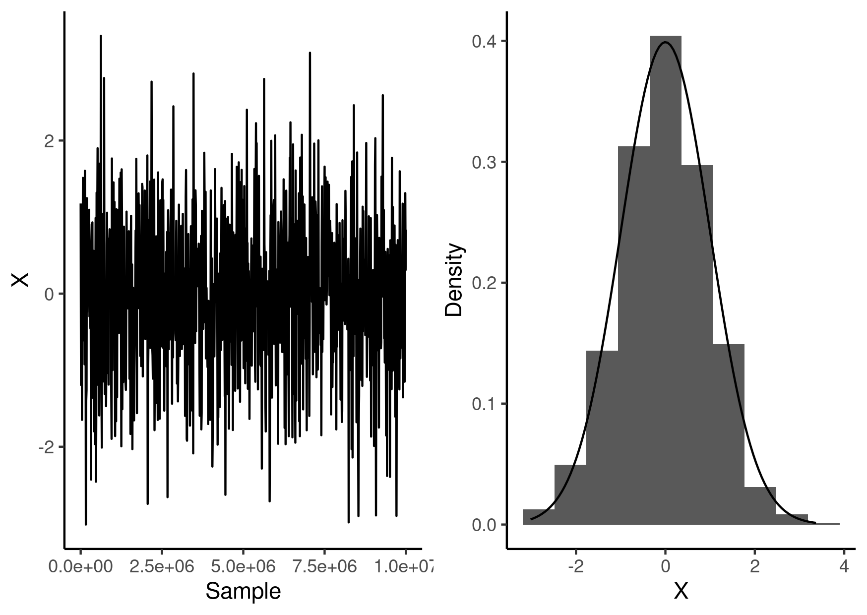
library(ggplot2)
library(cowplot)

beast_samples <- read.table("beast.csv",
  sep = "\t",
  comment.char = "#",
  header = TRUE
)

g1 <- ggplot() +
  geom_line(
    data = beast_samples,
    mapping = aes(x = Sample, y = x)
  ) +
  labs(x = "Sample", y = "X") +
  theme_classic()

g2 <- ggplot() +
  geom_histogram(
    data = beast_samples,
    mapping = aes(x = x, y = ..density..),
    bins = 10
  ) +
  stat_function(
    fun = \(x) dnorm(x),
    geom = "line"
  ) +
  labs(x = "X", y = "Density") +
  theme_classic()

g <- plot_grid(g1, g2)

ggsave("beast-demo.png",
       g,
       height = 10.5,
       width = 14.8,
       units = "cm")

BEAST2 as an MCMC engine: part II

This example looks at estimating the probability of heads in coin flips. We start with at beta prior distribution and take values of the number of observed heads and tails from the command line.

<?xml version="1.0" encoding="UTF-8" standalone="no"?>
<beast version="2.0">

    <distribution id="posterior" spec="beast.core.util.CompoundDistribution" >
        <distribution id="prior" spec="beast.math.distributions.Prior" x="@p">
            <distr spec="beast.math.distributions.Beta" alpha="0.5" beta="0.5" />
        </distribution>

        <distribution id="likelihood" spec="beast.math.distributions.Prior" x="@p">
            <distr spec="beast.math.distributions.Beta" alpha="$(heads)" beta="$(tails)" />
        </distribution>
    </distribution>

    <run chainLength="10000000" id="mcmc" preBurnin="100" spec="beast.core.MCMC">

        <state id="state" storeEvery="1000">
            <parameter estimate="true" id="p" name="stateNode" value="0.5" />
        </state>

        <distribution idref="posterior" />

        <operator spec="beast.evolution.operators.RealRandomWalkOperator" windowSize="0.1" useGaussian="true" weight="1.0" parameter="@p" />

        <logger id="screenlog" logEvery="1000000">
            <log idref="p" />
        </logger>

        <logger fileName="beast-02.csv" id="tracelog" logEvery="10000" model="@posterior">
            <log idref="posterior" />
            <log idref="p" />
        </logger>

    </run>

</beast>

Running the sampler

Here is the command to actually run this program.

java -jar beast.jar -seed 1 -overwrite -D "heads=3,tails=7" example-02.xml

The -D flag has been used to specify how many times the coin came up heads and tails.

Visualising the results

Here is a visualisation of the resulting samples along with the distribution we were sampling from.

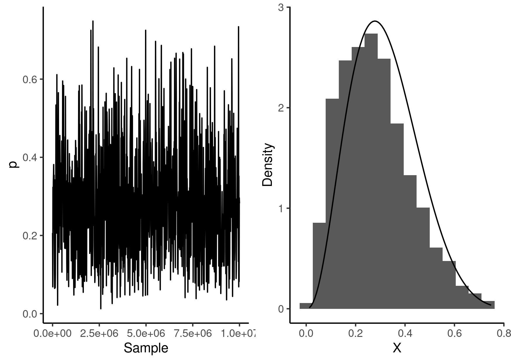
library(ggplot2)
library(cowplot)

beast_samples <- read.table("beast-02.csv",
  sep = "\t",
  comment.char = "#",
  header = TRUE
)

g1 <- ggplot() +
  geom_line(
    data = beast_samples,
    mapping = aes(x = Sample, y = p)
  ) +
  labs(x = "Sample", y = "p") +
  theme_classic()

g2 <- ggplot() +
  geom_histogram(
    data = beast_samples,
    mapping = aes(x = p, y = ..density..),
    bins = 15
  ) +
  stat_function(
    fun = \(x) dbeta(x, 0.5 + 3, 0.5 + 7),
    geom = "line"
  ) +
  labs(x = "X", y = "Density") +
  theme_classic()

g <- plot_grid(g1, g2)

ggsave("beast-02.png",
       g,
       height = 10.5,
       width = 14.8,
       units = "cm")

Birth-death simulation: Example I

In this example we will simulate sequences on a realisation of the birth-death process and then attempt to estimate the birth rate from these sequences. We will use ape to simulate the birth-death process and phangorn to simulate the sequences. To ensure a correct XML specification we will use beauti to generate the XML for the analysis. Finally, we will use tracer to check the results.

Simulating the tree

We will use years as our unit of time. Assuming that an individual is infectious for 7 days (\(1/52\) of a year) on average, and that \(1\%\) of infections are sequenced we end up with the following equations for the rates: \(\mu + \psi = 52\) and \(\psi / (\psi + \mu) = 1 / 100\). Solving these give us \(\mu = 5148/100\) and \(\psi = 52/100\). If we have an \(\lambda / (\mu + \psi) = R_{0} = 2\) then \(\lambda = 104\).

birth_rate <- 104
death_rate <- 5148 / 100
sampling_rate <- 52 / 100
sim_duration <- 0.15 # year

The rlineage function returns a realisation of the birth-death process as a phylo object.

net_removal_rate <- death_rate + sampling_rate
sim_tree <- rlineage(birth_rate,
                     net_removal_rate,
                     Tmax = sim_duration)

We include the tip dates as part of the tip labels because it makes it much easier to read the data into Beauti if you can parse this information from the top labels.

num_tips <- length(sim_tree$tip.label)
tip_fwd_times <- node.depth.edgelength(sim_tree)[1:num_tips]
sim_tree$tip.label <- sprintf("%s_%f",
                              sim_tree$tip.label,
                              2021 + tip_fwd_times)

The reconstructed tree is the tree that remains when we sample the extinct tips (ie those that are not extant). The probability that a tip is sequenced is \(\psi / (\mu + \psi\)\).

extant_mask <- tip_fwd_times >= sim_duration
num_removed <- sum(!extant_mask)
num_sampled <- rbinom(n = 1,
                      size = num_removed,
                      prob = sampling_rate / net_removal_rate)
sampled_tips <- sample(x = sim_tree$tip.label[!extant_mask],
                       size = num_sampled)
reconstructed_tree <- keep.tip(phy = sim_tree,
                               tip = sampled_tips)

We can combine all of this into a function

rand_reconstructed_tree <- function(birth_rate,
                                    death_rate,
                                    sampling_rate,
                                    duration) {
  net_removal_rate <- death_rate + sampling_rate
  sim_tree <- rlineage(birth_rate,
                       net_removal_rate,
                       Tmax = sim_duration)

  num_tips <- length(sim_tree$tip.label)
  tip_fwd_times <- node.depth.edgelength(sim_tree)[1:num_tips]
  sim_tree$tip.label <- sprintf("%s_%f",
                                sim_tree$tip.label,
                                2021 + tip_fwd_times)

  extant_mask <- tip_fwd_times >= sim_duration
  num_removed <- sum(!extant_mask)
  num_sampled <- rbinom(n = 1,
                        size = num_removed,
                        prob = sampling_rate / net_removal_rate)
  sampled_tips <- sample(x = sim_tree$tip.label[!extant_mask],
                         size = num_sampled)
  reconstructed_tree <- keep.tip(phy = sim_tree,
                                 tip = sampled_tips)

  return(reconstructed_tree)
}

We want a simulation that has a reasonable number of sequences in it, so we generate random trees until we have one with at least \(20\) tips.

iter_count <- 0
num_seqs <- 0
while (iter_count < 100 && num_seqs < 20) {
  reconstructed_tree <- rand_reconstructed_tree(birth_rate,
                                                death_rate,
                                                sampling_rate,
                                                sim_duration)
  iter_count <- iter_count + 1
  num_seqs <- length(reconstructed_tree$tip.label)
  print(iter_count)
}

This tree should be saved for later use.

write.tree(phy = reconstructed_tree,
           file = "reconstructed-tree.newick")

Simulating the sequences

Then we use the simSeq function to simulate a set of genomes for the leaves of this tree. By default this function uses the JC model for the sequence simulation with a rate of 1 (using the branch lengths as the units of time). RNA viruses have a mutation rate of \(\approx 10^{-3}\) substitutions per site per year. We are already working in units of years so we can use this as our rate. The length of the sequence we will use is 2000 which is similar to the HA of influenza.

sim_seqs <- simSeq(x = reconstructed_tree,
                   rate = 1e-3,
                   l = 2000,
                   type = "DNA")

Then we write this to a file so we can read it into Beauti.

write.phyDat(x = sim_seqs,
             file = "sequences.fasta",
             format = "fasta")

Constructing the XML

java -cp ~/Documents/beast2/build/dist/beast.jar beast.app.beauti.Beauti

Open Beauti and load in the alignment produced by the simulation above.
Open the Tip Dates tab and auto-configure to get the tip dates.
- Since the sequences have been simulated with JC model with rate 1 nothing special is needed for the Site Model and Clock Model tabs.
Open the Priors tab and select the Birth Death Skyline Serial prior
- The reproduction number has dimension 10 by default, we used constant rates so this should be reduced to 1.
- Go over the parameters and make sure that for each one the prior looks sensible. To make things a bit easier, set informative priors for each parameter.
Save the analysis as an XML.

Running the sampler

Running the sampler for \(10^{6}\) iterations does not take very long and allows us to see which variables are getting stuck. There are some suggested adjustments to the operators which should be done before increasing the sample size to \(10^{7}\).

Analysing the posterior samples

Tracer can be used for preliminary investigation of the posterior samples as shown in the following table (generated using tracer-table).

Summary Statistic	Mean	95% HPD Interval	Effective Sample Size
clock rate	7.641E-4	[3.9092E-4, 1.171E-3]	496.5
origin time	0.1509	[0.1146, 0.1935]	254.7
become uninfectious rate	51.9713	[50.0723, 53.9649]	4406.5
reproductive number	2.0901	[1.8752, 2.3189]	581.7
sampling proportion	0.0204	[1.9394E-3, 0.0435]	116.5

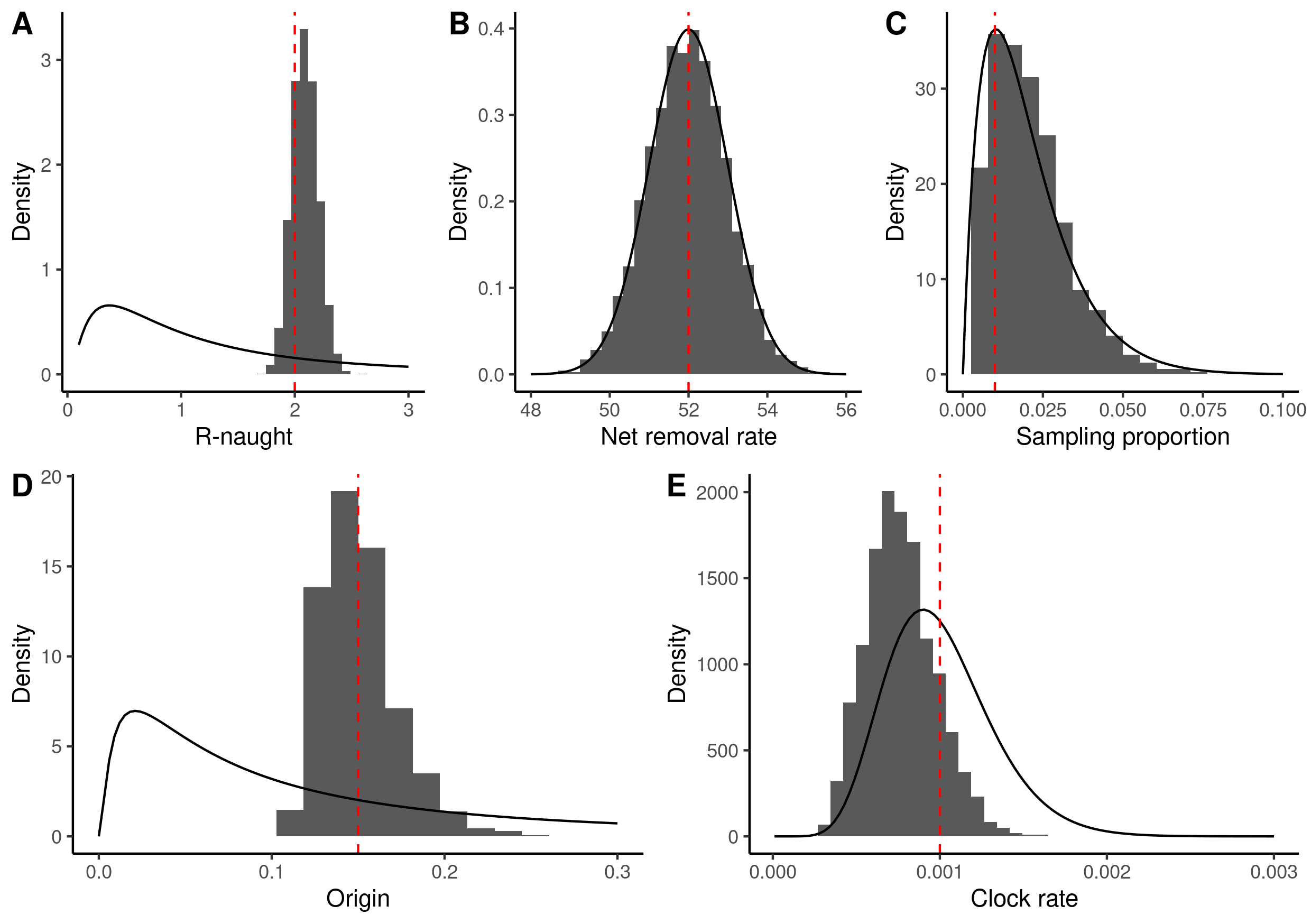
To display the prior and posteriors on the same figure we need to resort to ggplot2 though. There appear to be some identifiability issues (which is to be expected), but the estimates of the origin and basic reproduction number are decent. The figure shows the prior distributions (solid lines), the marginal posterior distribution (histogram) and the true values used in the simulation (dashed red line).

library(dplyr)
library(ggplot2)
library(magrittr)
library(purrr)
library(cowplot)

<<define-parameters>>

mcmc_samples <- read.csv(
  "sequences.log",
  comment.char = "#",
  sep = "\t"
) |>
  rename(
    clock_rate = clockRate,
    origin = origin_BDSKY_Serial,
    net_removal_rate = becomeUninfectiousRate_BDSKY_Serial,
    r_naught = reproductiveNumber_BDSKY_Serial,
    sampling_proportion = samplingProportion_BDSKY_Serial
  ) |>
  select(
    clock_rate,
    origin,
    net_removal_rate,
    r_naught,
    sampling_proportion
  ) |>
  tail(-1000)


g1 <- ggplot() +
  geom_histogram(
    data = mcmc_samples,
    mapping = aes(x = r_naught, y = ..density..),
    bins = 40
  ) +
  stat_function(
    fun = function(x) dlnorm(x, meanlog = 0.0, sdlog = 1.0),
    geom = "line"
  ) +
  geom_vline(
    xintercept = birth_rate / (death_rate + sampling_rate),
    linetype = "dashed",
    colour = "red"
  ) +
  xlim(c(0.1, 3)) +
  labs(x = "R-naught", y = "Density") +
  theme_classic()

g2 <- ggplot() +
  geom_histogram(
    data = mcmc_samples,
    mapping = aes(
      x = net_removal_rate,
      y = ..density..
    )
  ) +
  stat_function(
    fun = function(x) dnorm(x, mean = 52, sd = 1.0),
    geom = "line"
  ) +
  geom_vline(
    xintercept = death_rate + sampling_rate,
    linetype = "dashed",
    colour = "red"
  ) +
  xlim(c(48, 56)) +
  labs(x = "Net removal rate", y = "Density") +
  theme_classic()

g3 <- ggplot() +
  geom_histogram(
    data = mcmc_samples,
    mapping = aes(x = sampling_proportion, y = ..density..),
    bins = 20
  ) +
  stat_function(
    fun = function(x) dbeta(x, shape1 = 2.0, shape2 = 97.0),
    geom = "line"
  ) +
  geom_vline(
    xintercept = sampling_rate / (death_rate + sampling_rate),
    linetype = "dashed",
    colour = "red"
  ) +
  xlim(c(0, 0.1)) +
  labs(x = "Sampling proportion", y = "Density") +
  theme_classic()

g4 <- ggplot() +
  geom_histogram(
    data = mcmc_samples,
    mapping = aes(x = origin, y = ..density..),
    bins = 20
  ) +
  stat_function(
    fun = function(x) dlnorm(x, meanlog = log(0.1), sdlog = 1.25),
    geom = "line"
  ) +
  geom_vline(
    xintercept = sim_duration,
    linetype = "dashed",
    colour = "red"
  ) +
  xlim(c(0, 0.3)) +
  labs(x = "Origin", y = "Density") +
  theme_classic()

g5 <- ggplot() +
  geom_histogram(
    data = mcmc_samples,
    mapping = aes(x = clock_rate, y = ..density..),
    bins = 40
  ) +
  stat_function(
    fun = function(x) dgamma(x, 10, 1e4),
    geom = "line"
  ) +
  geom_vline(
    xintercept = 1e-3,
    linetype = "dashed",
    colour = "red"
  ) +
  xlim(c(1e-5, 3e-3)) +
  labs(x = "Clock rate", y = "Density") +
  theme_classic()

g_comb <- plot_grid(
  plot_grid(g1, g2, g3, nrow = 1, labels = LETTERS[1:3]),
  plot_grid(g4, g5, nrow = 1, labels = LETTERS[4:5]),
  nrow = 2
)

ggsave(
  filename = "combined-results.png",
  plot = g_comb,
  height = 14.8, width = 21.0,
  units = "cm"
)

Birth-death simulation: Example II

In this example we will do pretty much the same thing as above, but will simulate a second smaller epidemic in a different location where the sampling proportion is two-thirds of the size. The goal it to analyse the two datasets simultaneously to get tighter estimates on the common parameters but also get the individual parameters.

<<import-libraries>>

birth_rate <- 104
death_rate <- 5148 / 100
sampling_rate_1 <- 52 / 100
sampling_rate_2 <- 0.66 * 52 / 100
sim_duration <- 0.15 # year

<<define-random-sampler>>

iter_count <- 0
num_seqs <- 0
while (iter_count < 100 && num_seqs < 20) {
  reconstructed_tree_1 <- rand_reconstructed_tree(
    birth_rate,
    death_rate,
    sampling_rate_1,
    sim_duration)
  iter_count <- iter_count + 1
  num_seqs <- length(reconstructed_tree_1$tip.label)
}

write.tree(phy = reconstructed_tree_1,
           file = "reconstructed-tree-1.newick")

sim_seqs_1 <- simSeq(x = reconstructed_tree_1,
                     rate = 1e-3,
                     l = 2000,
                     type = "DNA")

write.phyDat(x = sim_seqs_1,
             file = "sequences-1.fasta",
             format = "fasta")

iter_count <- 0
num_seqs <- 0
while (iter_count < 100 && num_seqs < (0.66 * 20)) {
  reconstructed_tree_2 <- rand_reconstructed_tree(
    birth_rate,
    death_rate,
    sampling_rate_2,
    sim_duration)
  iter_count <- iter_count + 1
  num_seqs <- length(reconstructed_tree_2$tip.label)
}

write.tree(phy = reconstructed_tree_2,
           file = "reconstructed-tree-2.newick")

sim_seqs_2 <- simSeq(x = reconstructed_tree_2,
                     rate = 1e-3,
                     l = 2000,
                     type = "DNA")

write.phyDat(x = sim_seqs_2,
             file = "sequences-2.fasta",
             format = "fasta")

The resulting sequences can be given to Beauti and we can ask it to link the genetic models. The generated XML has different tree priors but we want to link the reproduction number and the becoming uninfectious rate and clock rate across the two datasets so a bit of care needs to be taken to ensure that there is only a single parameter for each of these things defined and that it is reused and only has a single prior.

To ensure a fair comparison with the previous analysis we can copy the prior specifications over. Although in doing this some minor tweaks need to be made to ensure that every ID is unique.

Running the analysis and looking at the estimates in Tracer we get the following table of estimates and HPDs which are very similar to those from the previous analysis which is perhaps not that surprising given we haven't added all that much additional data and the estimates were already tight. Note that the ratio of sampling proportions is close to the true ratio.

Summary Statistic	Mean	95% HPD Interval	Effective Sample Size (ESS)
clock rate	9.1163E-4	[5.2452E-4, 1.3203E-3]	845.3
origin time 1	0.1455	[0.1139, 0.1847]	378.6
origin time 2	0.1417	[0.1024, 0.1872]	516
become uninfectious rate	52.0074	[50.0846, 54.0113]	8307.3
reproductive number	2.1148	[1.9335, 2.3078]	836.8
sampling proportion 1	0.024	[4.511E-3, 0.0504]	92
sampling proportion 2	0.0146	[1.0711E-3, 0.033]	437.3

Simulating sequences

The following XML will simulate sequences for the taxons in the data tag based on a tree read from a Newick file (this requires feast to be installed.) The results are written to an XML because they take the form of a data block that you might use in subsequent analyses.

<beast version='2.0' namespace='beast.base.evolution.alignment:beast.pkgmgmt:beast.base.core:beast.base.inference:beast.base.evolution.tree.coalescent:beast.pkgmgmt:beast.base.core:beast.base.inference.util:beast.evolution.nuc:beast.base.evolution.operator:beast.base.inference.operator:beast.evolution.sitemodel:beast.evolution.substitutionmodel:beast.base.evolution.likelihood'>


    <data id="alignment" dataType="nucleotide">
        <sequence taxon="human">?</sequence>
        <sequence taxon="chimp">?</sequence>
        <sequence taxon="bonobo">?</sequence>
        <sequence taxon="gorilla">?</sequence>
        <sequence taxon="orangutan">?</sequence>
        <sequence taxon="siamang">?</sequence>
    </data>


    <tree spec='feast.fileio.TreeFromNewickFile' fileName="demo-tree.newick" IsLabelledNewick="true" adjustTipHeights="false" id='tree' />


    <run spec="beast.app.seqgen.SequenceSimulator" id="seqgen" data='@alignment' tree='@tree' sequencelength='100' outputFileName="demo-seqgen-output.xml">
        <siteModel spec='SiteModel'>
            <substModel spec='JukesCantor' />
        </siteModel>

        <branchRateModel id="StrictClock" spec="beast.evolution.branchratemodel.StrictClockModel">
            <parameter dimension="1" estimate="false" id="clockRate" minordimension="1" name="clock.rate" value="1.0" />
        </branchRateModel>

    </run>
</beast>

beast2-aez-notes

Table of Contents

Links

Notes

Understanding BEAUti

Build a BEAST2

Notes

TODO Understanding Packages

Installing packages from source

TODO Configuring IntelliJ for writing a package

Understanding BEAST2

Packages provided by BEAST2

Understanding bdsky

Understanding the XML

The plate macro

Understanding the MCMC application

Starting tree

Priors

Operators

Tuning operators

Simulating data

MASTER

Piece-wise constant rates

Tools and useful R functions

Cogsworth

Web beautify

Read BEAST2 log file

Pretty printing Tracer output

Examples

BEAST2 as an MCMC engine: part I

The target distribution

MCMC

Running the sampler

Visualising the results

BEAST2 as an MCMC engine: part II

Running the sampler

Visualising the results

Birth-death simulation: Example I

Simulating the tree

Simulating the sequences

Constructing the XML

Running the sampler

Analysing the posterior samples

Birth-death simulation: Example II

Simulating sequences

Understanding `bdsky`