AANN 03/01/2024

Basic model using PyTorch for MNIST classification

In this example we use a very simple feed-forward neural network for handwritten digit recognition. This gets an accuracy on the test dataset of \(97\%\).

We use the MNISTDataset (which is a map-style subclass of Dataset) to store the data in memory. This enables us to use the DataLoader class which simplifies batching and shuffling of the data. The batching substantially speeds up the evaluation.

import torch
import torch.nn as nn
import torch.optim as optim
import numpy as np
import pandas as pd
import plotnine as p9
from plotnine import *

import niceneuron.io as nn_io
import niceneuron.data as nn_data
import niceneuron.plot as nn_plot

loss_csv = "example-2024-01-03-loss.csv"
loss_png = "example-2024-01-03-loss.png"

# Load the MNIST training dataset
images_path = 'data/train-images.idx3-ubyte'
labels_path = 'data/train-labels.idx1-ubyte'
images = nn_io.read_idx(images_path)
assert images.min() == 0 and images.max() == 255
images = images / 255.0 # Normalize pixel values to be between 0 and 1
images = images.astype(np.float32)
labels = nn_io.read_idx(labels_path)

train_dataset = nn_data.MNISTDataset(images, labels)
train_dataloader = torch.utils.data.DataLoader(train_dataset, batch_size=64, shuffle=True)

# Load the MNIST test dataset
test_images_path = 'data/t10k-images.idx3-ubyte'
test_labels_path = 'data/t10k-labels.idx1-ubyte'
test_images = nn_io.read_idx(test_images_path)
assert test_images.min() == 0 and test_images.max() == 255
test_images = test_images / 255.0 # Normalize pixel values to be between 0 and 1
test_images = test_images.astype(np.float32)
test_labels = nn_io.read_idx(test_labels_path)
test_dataset = nn_data.MNISTDataset(test_images, test_labels)
test_dataloader = torch.utils.data.DataLoader(test_dataset, batch_size=64, shuffle=False)

Here we define the neural network we will use with the DemoModel class.

class DemoModel(nn.Module):
    def __init__(self):
        super(DemoModel, self).__init__()
        self.dense_layers = nn.Sequential(
            nn.Linear(28*28, 128),
            nn.ReLU(),
            nn.Linear(128, 10)
        )

    def forward(self, x):
        logits = self.dense_layers(x)
        return logits


model = DemoModel()

Then we need to define a training loop for the model.

# Train the model
loss_fn = nn.CrossEntropyLoss()
optimizer = optim.Adam(model.parameters(), lr=1e-3)

model.train()
loss_history = []
for epoch in range(5):
    epoch_cumloss = 0
    for image, label in train_dataloader:
        # Forward pass
        logits = model(image)
        loss = loss_fn(logits, label)
        epoch_cumloss += loss.item()

        # Backward pass
        optimizer.zero_grad()
        loss.backward()
        optimizer.step()

    print(f"Epoch {epoch} loss: {epoch_cumloss}")
    loss_history.append((epoch,epoch_cumloss))

loss_df = pd.DataFrame(loss_history, columns=['epoch', 'loss'])
loss_df.to_csv(loss_csv, index=False)

Then we test it with the following loop. Note that we have turned the gradient tracking off as this runs slightly quicker.

# Use the test dataset to evaluate the model
model.eval()
correct = 0
total = 0
with torch.no_grad():
    for image, label in test_dataloader:
        logits = model(image)
        predicted = torch.argmax(logits, dim=1)
        total += label.size(0)
        correct += (predicted == label).sum().item()

# print test accuracy
print(f"Test accuracy: {correct / total}")

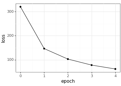
Plot the resulting loss values across the epochs.

loss_df = pd.read_csv(loss_csv)
loss_p9 = nn_plot.plot_loss_curve(loss_df)
loss_p9.save(loss_png, height = 2.9, width = 4.1)