AANN 04/01/2024

CNN using PyTorch for MNIST classification

In this example we use a simple convolutional neural network for handwritten digit recognition. This gets an accuracy on the test dataset of \(98\%\). That is better performance with a smaller model than in the previous example. The training took less than a minute on my laptop.

There is a nice explanation of CNNs here.

depth: The depth of the input volume is the number of channels, e.g. the RGB associated with a pixel. The depth of the output volume is the number of filters in the CNN.
stride: The number of pixels we move the filter at each step.
zero-padding: The depth of zero-padding around the image.
pooling: A layer included between convolutions that reduces the size of the volume by taking a summary (typically the max) over the spatial extent. A common choice is max pooling, a \(2\times 2\) filter with a stride of \(2\) and taking the max value.

Loading packages

import time
import torch
import torch.nn as nn
import torch.optim as optim
import numpy as np
import pandas as pd
import plotnine as p9
from plotnine import *

import niceneuron.io as nn_io
import niceneuron.data as nn_data

Define input and output filenames

Define the files that are used as input and output to keep the program DRY.

images_path = 'data/train-images.idx3-ubyte'
labels_path = 'data/train-labels.idx1-ubyte'
test_images_path = 'data/t10k-images.idx3-ubyte'
test_labels_path = 'data/t10k-labels.idx1-ubyte'

loss_csv = "example-2024-01-04-loss.csv"
loss_png = "example-2024-01-04-loss.png"
trained_model_file = "example-2024-01-04-model.pt"

Loading testing and training data

images = nn_io.read_idx(images_path)
images = images.astype(np.float32)
labels = nn_io.read_idx(labels_path)

train_dataset = nn_data.MNISTDataset(
    images, labels, flatten=False, normalise=True)
train_dataloader = torch.utils.data.DataLoader(train_dataset, batch_size=64, shuffle=True)

test_images = nn_io.read_idx(test_images_path)
test_images = test_images.astype(np.float32)
test_labels = nn_io.read_idx(test_labels_path)
test_dataset = nn_data.MNISTDataset(
    test_images, test_labels, flatten=False, normalise=True)
test_dataloader = torch.utils.data.DataLoader(test_dataset, batch_size=64, shuffle=False)

Defining the model

Here we define the neural network we will use with the DemoCNN class.

class DemoCNN(nn.Module):
    def __init__(self):
        super(DemoCNN, self).__init__()
        self._conv1 = nn.Conv2d(1, 6, kernel_size=5, padding=2)
        self._pool1 = nn.AvgPool2d(2)
        self._conv2 = nn.Conv2d(6, 16, kernel_size=5, padding=0)
        self._pool2 = nn.AvgPool2d(2)
        self._fc1 = nn.Linear(5*5*16, 84)
        self._fc2 = nn.Linear(84, 10)
        self._relu = nn.ReLU()

    def forward(self, x):
        x = self._pool1(self._relu(self._conv1(x)))
        x = self._pool2(self._relu(self._conv2(x)))
        x = x.view(-1, 5*5*16)
        x = self._relu(self._fc1(x))
        x = self._fc2(x)
        return x

Train the model

Then we need to define a training loop for the model.

model = DemoCNN()

loss_fn = nn.CrossEntropyLoss()
optimizer = optim.Adam(model.parameters(), lr=1e-3)

model.train()
loss_history = []
training_start_time = time.time()
for epoch in range(5):
    epoch_cumloss = 0
    for images, label in train_dataloader:
        images = images.unsqueeze(1)
        # Forward pass
        logits = model(images)
        loss = loss_fn(logits, label)
        epoch_cumloss += loss.item()

        # Backward pass
        optimizer.zero_grad()
        loss.backward()
        optimizer.step()

    print(f"Epoch {epoch} loss: {epoch_cumloss}")
    loss_history.append((epoch,epoch_cumloss))

training_finish_time = time.time()
print(f"Training took: {training_finish_time - training_start_time}")

loss_df = pd.DataFrame(loss_history, columns=['epoch', 'loss'])
loss_df.to_csv(loss_csv, index=False)

Saving the model

Instead of saving the nn.Module as a single object we just save the state of the model which is the recommendation from PyTorch.

torch.save(model.state_dict(), trained_model_file)

You could then reload this state later with a new instance of the model:

prev_state_dict = torch.load(trained_model_file)
new_model = DemoCNN()
new_model.load_state_dict(prev_state_dict)

Test the model

Then we test it with the following loop. Note that we have turned the gradient tracking off as this runs slightly quicker.

model.eval()
correct = 0
total = 0
with torch.no_grad():
    for images, label in test_dataloader:
        images = images.unsqueeze(1)
        logits = model(images)
        predicted = torch.argmax(logits, dim=1)
        total += label.size(0)
        correct += (predicted == label).sum().item()

# print test accuracy
print(f"Test accuracy: {correct / total}")

Visualise the results

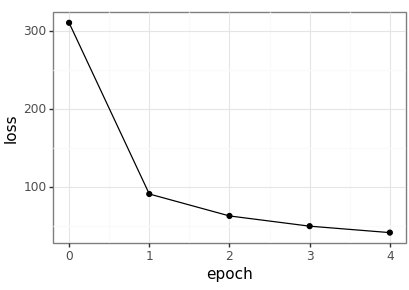
Plot the resulting loss values across the epochs.

loss_df = pd.read_csv(loss_csv)
loss_p9 = (
    ggplot(loss_df, aes(x='epoch', y='loss')) +
    geom_point() +
    geom_line() +
    theme_bw()
)
loss_p9.save(loss_png, height = 2.9, width = 4.1)