aez-notes

Examples
- Map of Italy using spatial data
- Annotation for a linear model
Installation and usage
- Saving figures to SVG
- Ggtree
Resources/references
Colophon

THE CONTENT OF THIS PAGE IS SLOWLY BEING MIGRATED TO A GALLERY OF EXAMPLES.

The friends include ggmap and ggtree and cowplot and ggspatial and latex2exp

To include latex in any sort of text on a figure there is the latex2exp package on CRAN which provides the TeX function. You can wrap most strings in this before passing to plotting code. The vignette for this package describes the expressions supported and has multiple examples.

Examples

Map of Italy using spatial data

Depending on the machine set up you may need to use convert to change a PDF of this map to a PNG.

library(ggplot2)
library(ggspatial)
library(GADMTools)
library(purrr)
library(dplyr)
library(reshape2)
library(ggmap)

## Define some parameters for how to draw and colour the figure

my_breaks <- c(0,5,10)

my_cols <- hcl.colors(n = length(my_breaks) - 1,
                      palette = "reds 3",
                      alpha = NULL,
                      rev = TRUE,
                      fixup = TRUE)

map_country_line_colour <- "#252525"
map_inline_thickness <- 0.1
map_outline_thickness <- 0.5

map_plot_background <- element_rect(colour = "#252525",
                                    fill = "#FFFFFF")


## Load the map data from GADM
italy_sf <- gadm_sf_loadCountries("ITA", level = 1)$sf
italy_sf$foobar <- rpois(n = nrow(italy_sf), lambda = 3)

## Include an additional level zero object for the country outline.
italy_outline_sf <- gadm_sf_loadCountries("ITA", level = 0)$sf



g <- ggplot() +
    geom_sf(data = italy_sf,
            mapping = aes(fill = foobar),
            colour = map_country_line_colour,
            size = map_inline_thickness) +
    geom_sf(data = italy_outline_sf,
            fill = NA,
            colour = map_country_line_colour,
            size = map_outline_thickness) +
    scale_fill_gradientn(breaks = my_breaks,
                         colors = my_cols,
                         limits = range(my_breaks)) +
    theme(plot.background = map_plot_background) +
    labs(fill = "Foobar") +
    theme_void() +
    theme(legend.position = "left")

ggsave("../resources/ggplot2-example-02.pdf",
       g)

Annotation for a linear model

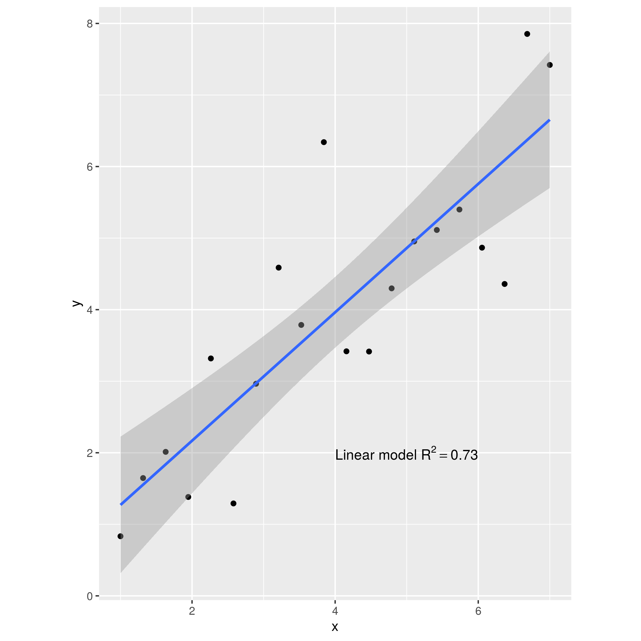
library(magrittr)
library(ggplot2)
library(latex2exp)


x <- seq(from = 1, to = 7, length = 20)
y <- rnorm(n = length(x), mean = x, sd = 1)
z <- data.frame(x = x, y = y)

rsquared <- lm(y ~ x, data = z) %>%
  summary %>%
  use_series("r.squared")

annotation_exp <- TeX(sprintf("Linear model $R^2 = %.2f$", rsquared))

g <- ggplot(data = z,
       mapping = aes(x = x, y = y)) +
  geom_point() +
  geom_smooth(method = "lm") +
  annotate(geom = "text",
           x = 5,
           y = 2,
           label = annotation_exp) +
  coord_fixed()

ggsave("../resources/ggplot2-example-05.png",
       g)

Installation and usage

Saving figures to SVG

To save a figute to an SVG using ggsave you need the svglite package to be installed. This in turn needs a Cairo library to be installed on your system. On Ubuntu, this requred me to install libcairo2-dev.

Ggtree

ggtree is not on CRAN but you can install it with Bioconductor.

if (!requireNamespace("BiocManager", quietly = TRUE))
  install.packages("BiocManager")

BiocManager::install("ggtree")

Resources/references

Colophon

The R scripts shown in this document can be tangled out and where run to generate the figures shown. This is done by running the following script in the following nix shell.

# run-ggplot2-examples.sh

for ix in `seq 1 6`;
do
    Rscript ggplot2-example-0$ix.R
done

# ggplot2-shell.nix 
let
  commitHash = "78dc359abf8217da2499a6da0fcf624b139d7ac3";
  tarballUrl = "https://github.com/NixOS/nixpkgs/archive/${commitHash}.tar.gz";
  pkgs = import (fetchTarball tarballUrl) {};
  stdenv = pkgs.stdenv;
in with pkgs; {
  myProject = stdenv.mkDerivation {
    name = "ggplot2-env";
    version = "1";
    src = if pkgs.lib.inNixShell then null else nix;

    buildInputs = with rPackages; [
      R
      rPackages.cowplot
      rPackages.dplyr
      rPackages.ggplot2
      rPackages.ggspatial
      rPackages.latex2exp
      rPackages.magrittr
      rPackages.purrr
      rPackages.stringi
      rPackages.udunits2
    ];
   shellHook = ''
             printf "\n\nWelcome to the ggplot2 shell :)\n\n"
      '';
  };
}