ggplot2 gallery
![]()
- colorbrewer2
- DataVisProject: a catalogue of visualisation types
- ggplot2 extensions
- R Graph Gallery
- R spatial blog posts
Gallery
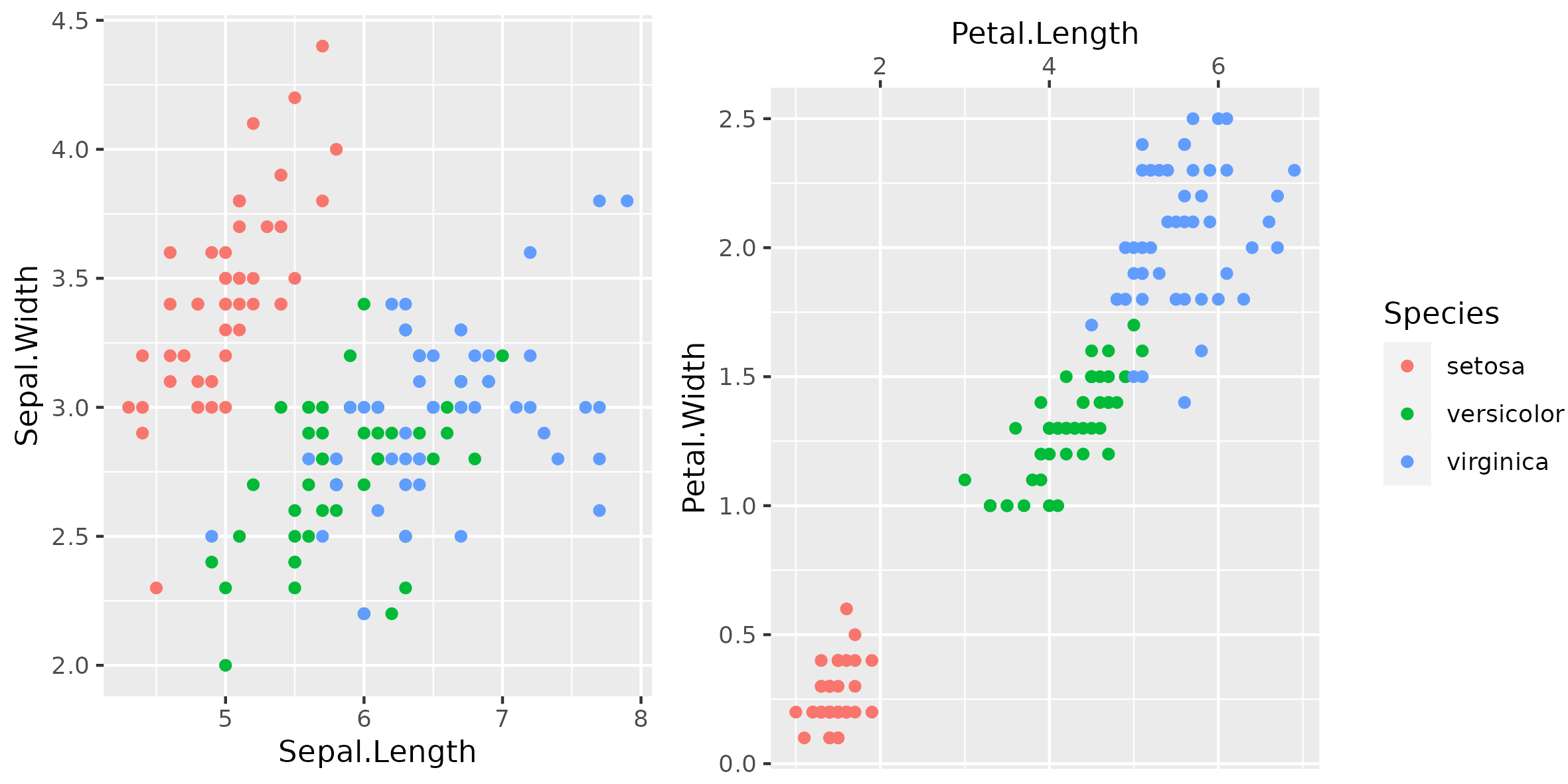
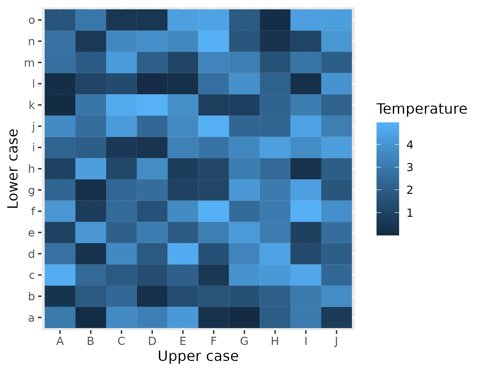
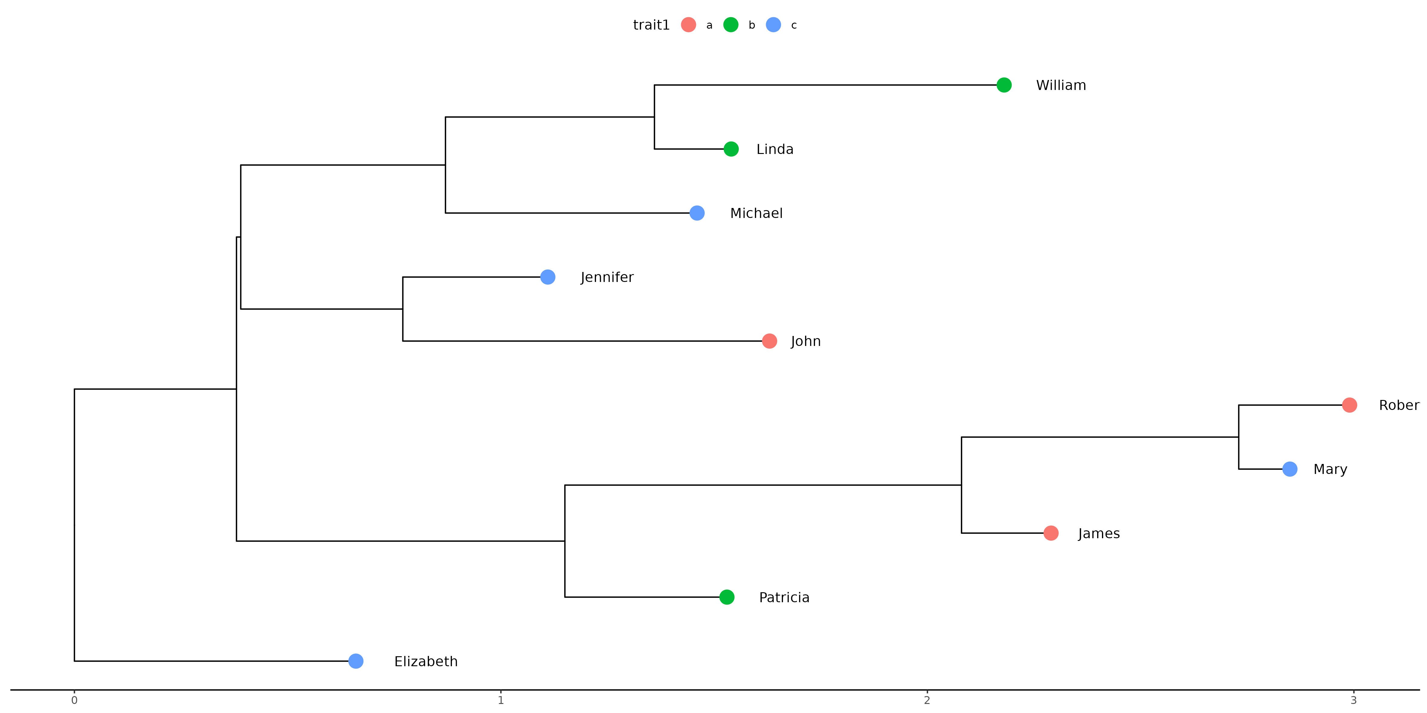
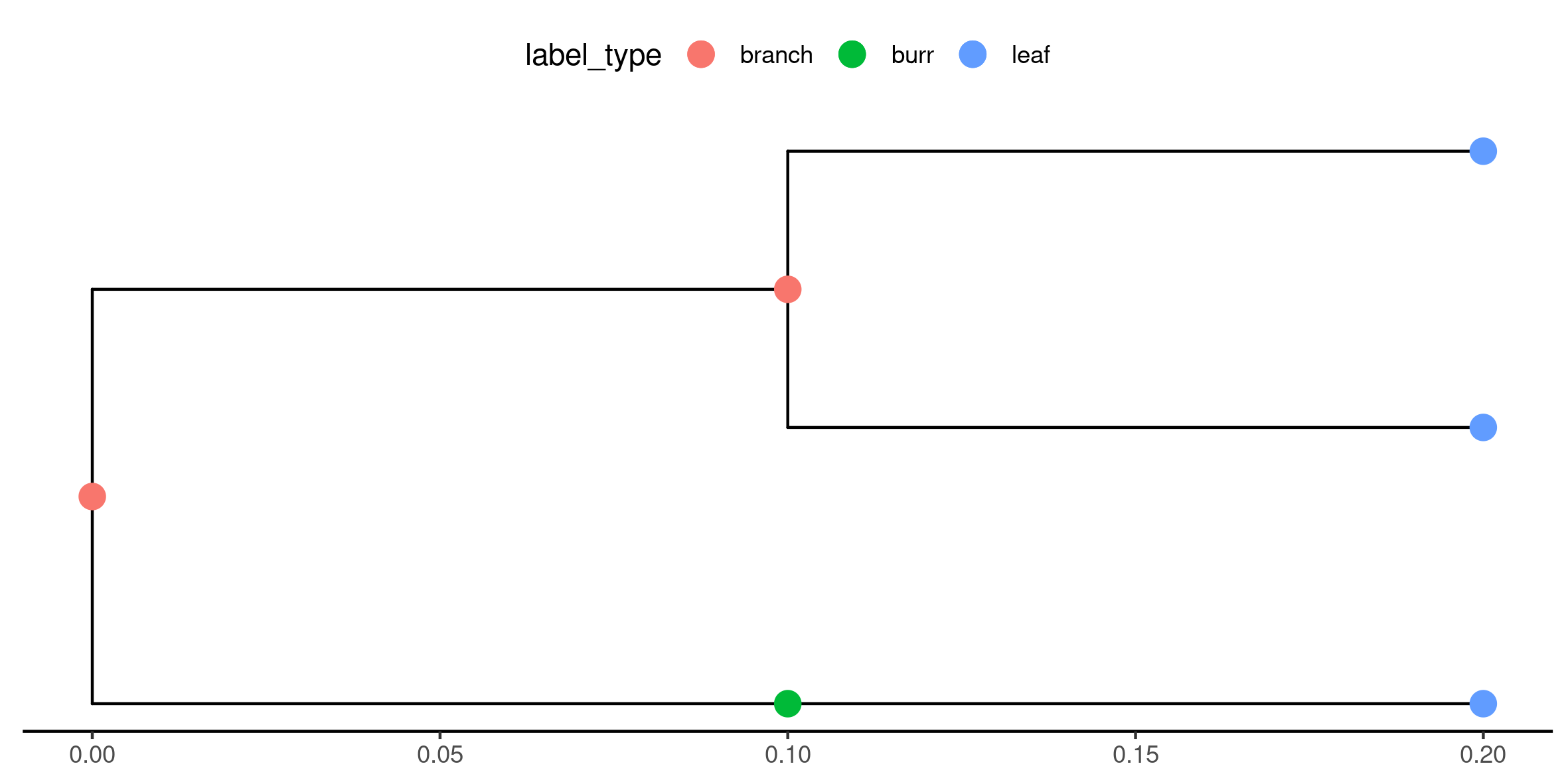
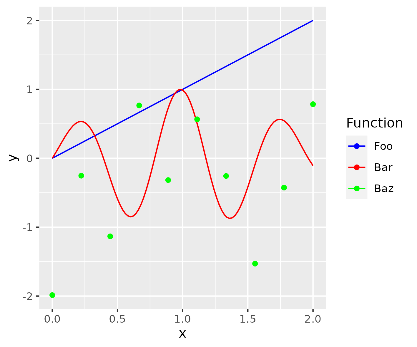
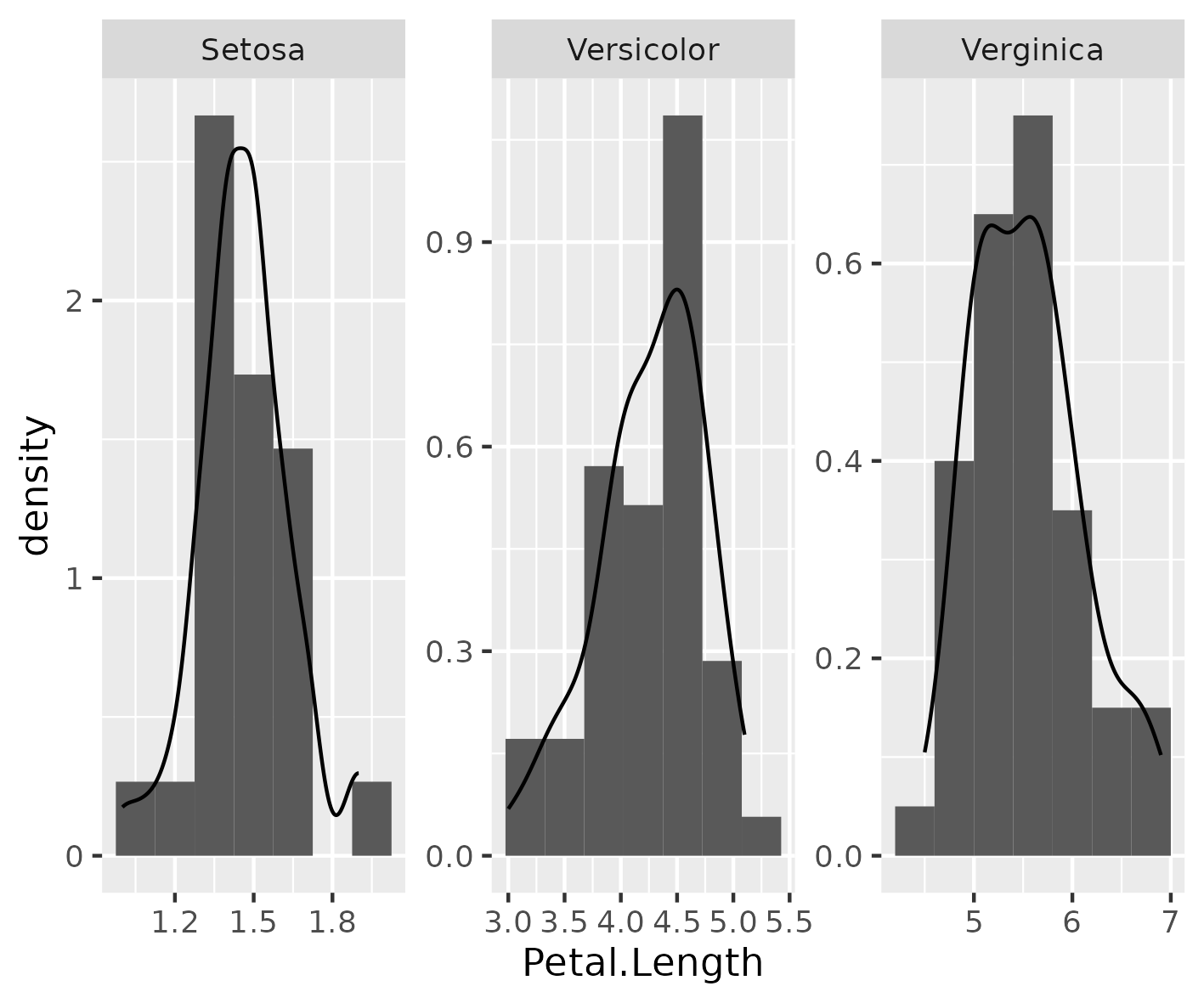
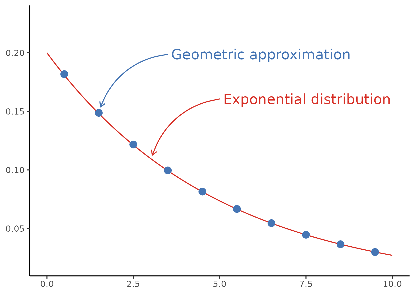
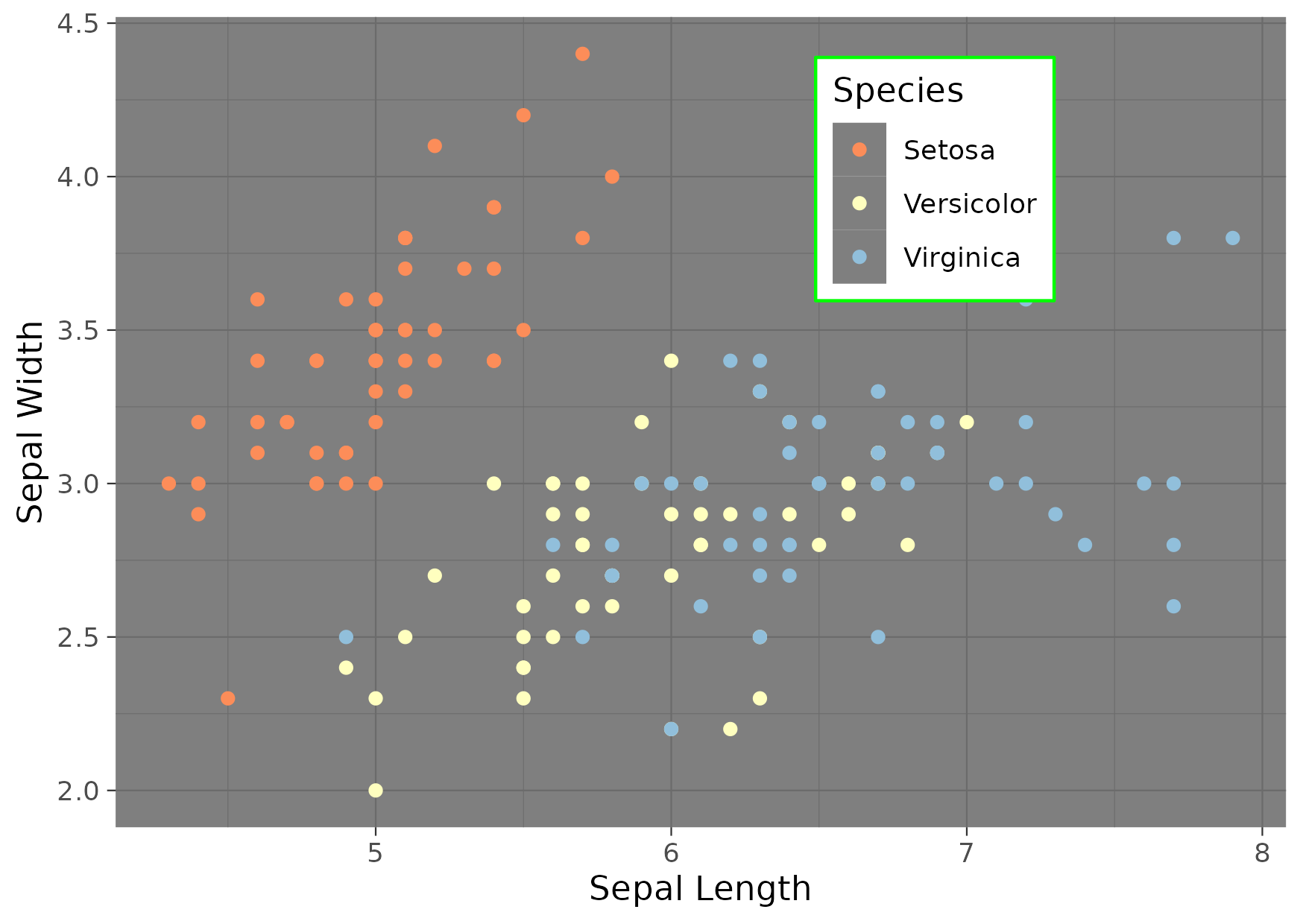

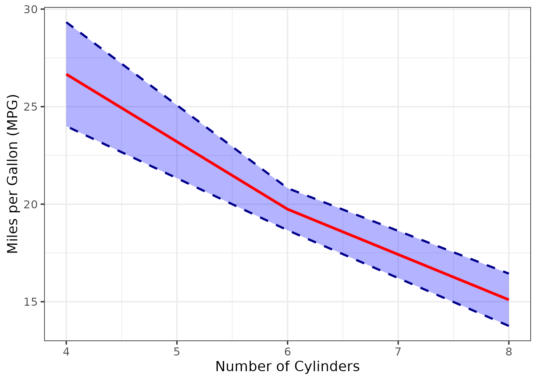
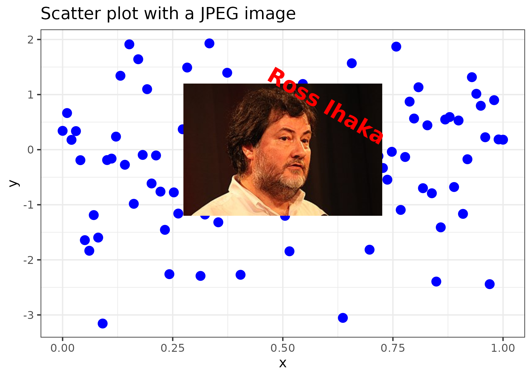
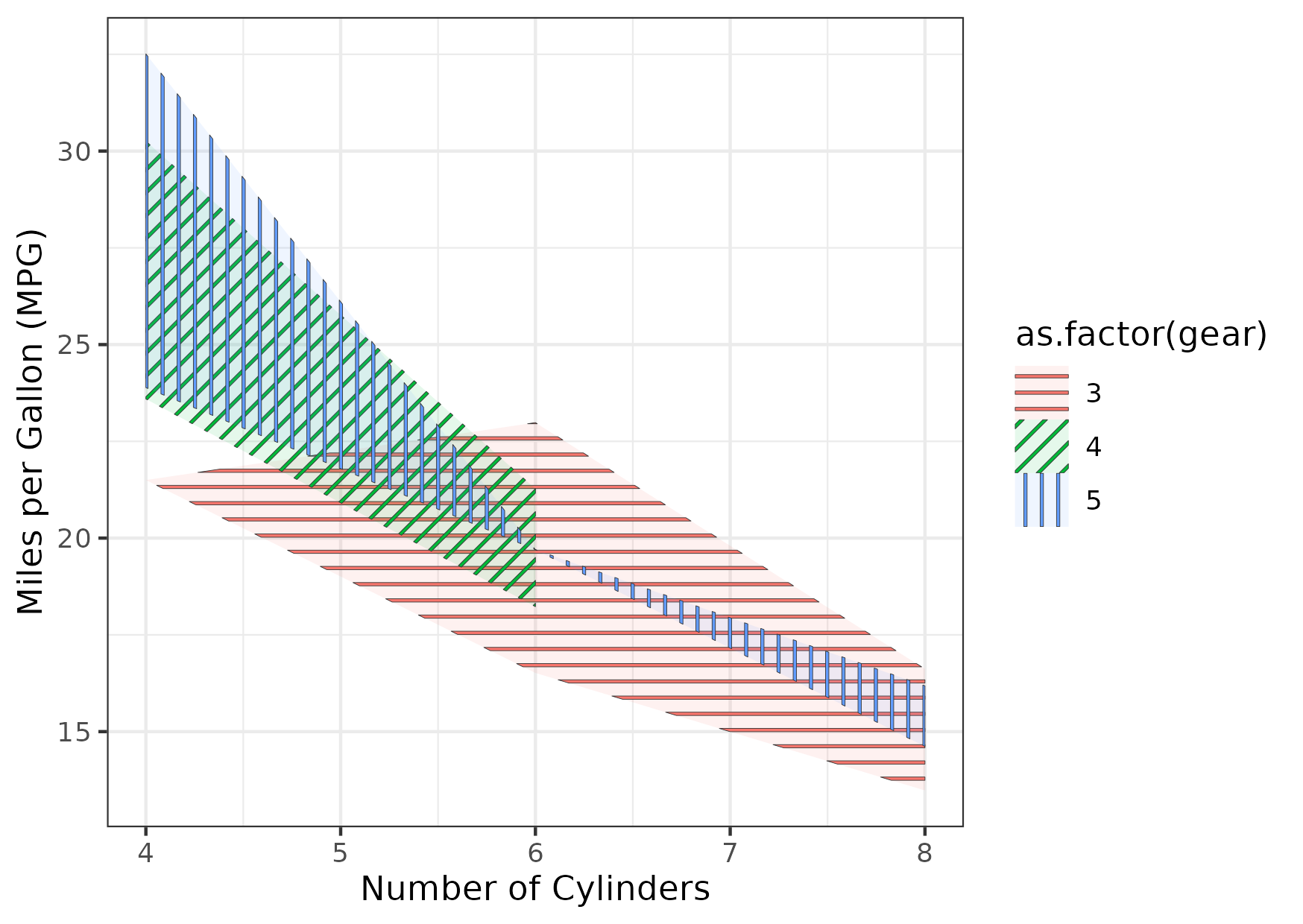
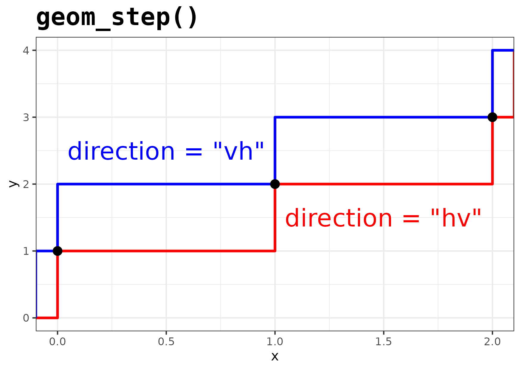
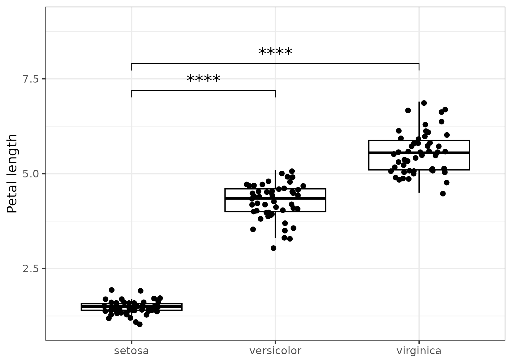
Figure 1
Keywords: cowplot, combining plots
library(ggplot2)
library(cowplot)

a <- ggplot() +
  geom_point(data = iris,
             mapping = aes(x = Sepal.Length,
                           y = Sepal.Width,
                           colour = Species))

b <- ggplot() +
  geom_point(data = iris,
             mapping = aes(x = Petal.Length,
                           y = Petal.Width,
                           colour = Species)) +
  scale_x_continuous(position = "top")

legend <- get_legend(b + theme(legend.box.margin = margin(0, 0, 0, 12)))

example_plot <-
  plot_grid(a + theme(legend.position = "none"),
            b + theme(legend.position = "none"),
            legend,
            ncol = 3,
            rel_widths = c(1, 1, 0.35))

ggsave("fig01.png",
       example_plot,
       width = 20,
       height = 10,
       units = "cm")
Figure 2
Keywords: heatmap, matrix, tile geometry
library(ggplot2)

x <- LETTERS[1:10]
y <- letters[1:15]
plot_df <- expand.grid(x=x, y=y)
plot_df$z <- runif(length(x) * length(y), 0, 5)

example_plot <- ggplot() +
  geom_tile(
    data = plot_df,
    mapping = aes(x = x, y = y, fill = z)
  ) +
  labs(
    x = "Upper case",
    y = "Lower case",
    fill = "Temperature")
  theme_minimal()

ggsave("fig02.png",
       example_plot,
       width = 13,
       height = 10,
       units = "cm")
Figure 3
Keywords: tree, phylogeny, ggtree, newick
library(ggplot2)
library(ggtree)
library(treeio)
library(tidytree)

set.seed(1)

newick_str <- "((((t7:0.21,(t2:0.12,t3:0.26):0.65):0.93,t8:0.38):0.77,((t1:0.86,t5:0.34):0.38,(t6:0.59,(t9:0.18,t10:0.82):0.49):0.48):0.01):0.38,t4:0.66);"

my_phylo <- read.tree(text = newick_str)

human_names <- c(
  "James",
  "Mary",
  "Robert",
  "Patricia",
  "John",
  "Jennifer",
  "Michael",
  "Linda",
  "William",
  "Elizabeth"
)

annotations <- tibble(
  node = seq.int(length(my_phylo$tip.label)),
  trait1 = sample(letters[1:3], 10, replace = TRUE),
  trait2 = human_names
)

my_tree <- treedata(phylo = my_phylo, data = annotations)

example_plot <- ggplot(my_tree, mapping = aes(x, y)) +
  geom_tree() +
  geom_tippoint(mapping = aes(colour = trait1),
                size = 5) +
  geom_tiplab(mapping = aes(label = trait2),
              hjust = -0.5) +
  theme_tree2(legend.position='top')

ggsave("fig03.png",
       example_plot,
       width = 40,
       height = 20,
       units = "cm")
Figure 4
Keywords: tree, phylogeny, ggtree, newick, annotation
library(ggplot2)
library(ggtree)
library(treeio)
library(tidytree)
library(tibble)
library(ape)

set.seed(1)

newick_str <- "((t1:0.1,t2:0.1):0.1,(t3:0.1)t4:0.1);"

leaf_names <- c("t1", "t2", "t3")
burr_names <- c("t4")

label_type <- function(label) {
  ifelse(
    is.element(label, leaf_names),
    "leaf",
  ifelse(
    is.element(label, burr_names),
    "burr",
    "branch")
  )
}

my_phylo_tbl <- as_tibble(read.tree(text = newick_str))

my_data_tbl <- tibble(
  node = my_phylo_tbl$node,
  label_type = label_type(my_phylo_tbl$label)
)


my_td <- as.treedata(
  full_join(my_phylo_tbl, my_data_tbl, by = "node")
)

example_plot <- ggplot(my_td, mapping = aes(x, y)) +
  geom_tree() +
  geom_tippoint(aes(colour = label_type), size = 4) +
  geom_nodepoint(aes(colour = label_type), size = 4) +
  theme_tree2(legend.position = "top")

ggsave("fig04.png",
       example_plot,
       width = 20,
       height = 10,
       units = "cm")
Figure 5
Keywords: function, curve, expression, colours
library(ggplot2)

example_plot <- ggplot(data.frame(x = c(0, 2)), aes(x)) +
  stat_function(
    fun = identity,
    geom = "line",
    mapping = aes(colour = "Foo")
  ) +
  stat_function(
    fun = function(x) exp(-(x - 1)^2) * sin(x * 8),
    geom = "line",
    mapping = aes(colour = "Bar")
  ) +
  geom_point(
    data = data.frame(
      x = seq(0, 2, length = 10),
      y = rnorm(10)
    ),
    mapping = aes(colour = "Baz", y = y)
  ) +
  scale_colour_manual("Function",
    values = c("blue", "red", "green"),
    breaks = c("Foo", "Bar", "Baz")
  )

ggsave("fig05.png",
       example_plot,
       width = 12,
       height = 10,
       units = "cm")
Figure 6
Keywords: facet labels
library(dplyr)
library(ggplot2)

plot_df <- iris %>% select(Petal.Length, Species)

facet_labels <- c(
  setosa = "Setosa",
  versicolor = "Versicolor",
  virginica = "Verginica"
)

example_plot <- ggplot(plot_df, aes(x = Petal.Length)) +
  geom_histogram(
    mapping = aes(y = ..density..),
    bins = 7
  ) +
  geom_density() +
  facet_wrap(~Species,
             scales = "free",
             labeller = labeller(Species = facet_labels)
             )

ggsave("fig06.png",
       example_plot,
       width = 12,
       height = 10,
       units = "cm")
Figure 7
Keywords: annotations, arrows, colours
library(ggplot2)
library(dplyr)

## Some hex codes to use as a colour scheme. These are from
## \code{https://colorbrewer2.org/?type=diverging&scheme=RdYlBu&n=7}
my_colours <- list(
  truth = list(dark = "#d73027", light = "#fee090"),
  estimate = list(dark = "#4575b4", light = "#e0f3f8")
)

exp_rate <- 0.2
x_max <- 10
xs <- seq(from = 0, to = x_max, length = 100)
pdf_xs <- dexp(x = xs, rate = exp_rate)

delta <- 1.0
p_hat <- 2 * exp_rate * delta / (exp_rate * delta + 2)

n_max <- ceiling(x_max / delta - 0.5)
ns <- seq.int(from = 0, to = n_max)
ys <- delta * (ns + 0.5)
pmf_ys <- dgeom(x = ns, prob = p_hat)

my_fig <- ggplot() +
    geom_line(
        data.frame(x = xs, y = pdf_xs),
        mapping = aes(x = x, y = y),
        colour = my_colours$truth$dark
    ) +
    geom_point(
        filter(data.frame(x = ys, y = pmf_ys), x < x_max),
        mapping = aes(x = x, y = y),
        colour = my_colours$estimate$dark,
        size = 3
    ) +
    annotate(
        geom = "curve",
        xend = ys[2] + 0.05, yend = pmf_ys[2] + 0.005,
        x = ys[2] + 2, y = pmf_ys[2] + 0.05,
        curvature = 0.3,
        arrow = arrow(length = unit(2, "mm")),
        colour = my_colours$estimate$dark
    ) +
    annotate(
        geom = "text",
        x = ys[2] + 2 + 0.10, y = pmf_ys[2] + 0.05,
        label = "Geometric approximation",
        hjust = "left",
        colour = my_colours$estimate$dark,
        size = 5
    ) +
    annotate(
        geom = "curve",
        xend = 0.5*(ys[3] + ys[4]) + 0.05, yend = 0.5*(pmf_ys[3] + pmf_ys[4]) + 0.002,
        x = 0.5*(ys[3] + ys[4]) + 2, y = 0.5*(pmf_ys[3] + pmf_ys[4]) + 0.05,
        curvature = 0.3,
        arrow = arrow(length = unit(2, "mm")),
        colour = my_colours$truth$dark
    ) +
    annotate(
        geom = "text",
        x = 0.5*(ys[3] + ys[4]) + 2 + 0.10, y = 0.5*(pmf_ys[3] + pmf_ys[4]) + 0.05,
        label = "Exponential distribution",
        hjust = "left",
        colour = my_colours$truth$dark,
        size = 5
    ) +
    ylim(c(0.02, 0.23)) +
    theme_classic() +
    theme(axis.title = element_blank())

ggsave(filename = "fig07.png",
       plot = my_fig,
       height = 10.5, width = 14.8,
       units = "cm")
Figure 8
Keywords: Scales, colours, legends
library(ggplot2)

hex_cols <- c('#fc8d59','#ffffbf','#91bfdb')

gg <-
  ggplot() +
  geom_point(
    data = iris,
    mapping = aes(x = Sepal.Length,
                  y = Sepal.Width,
                  colour = Species)
  ) +
  scale_color_manual(
    values = hex_cols,
    breaks = c("setosa", "versicolor", "virginica"),
    labels = c("Setosa", "Versicolor", "Virginica")
  ) +
  labs(
    x = "Sepal Length",
    y = "Sepal Width"
  ) +
  theme_dark() +
  theme(
    legend.background = element_rect(fill = "white", colour = "green"),
    legend.position = c(0.7, 0.8)
  )

ggsave("fig08.png",
       gg,
       height = 10.5, width = 14.8,
       units = "cm")
Figure 0
Keywords: geometries, ribbons, step, helper
library(ggplot2)

#' Make a data frame for a ribbon step plot
#'
#' @param xs x values
#' @param ymins y minimum values
#' @param ymaxs y maximum values
#'
#' @examples
#' plot_df <- make_ribbonstep_df(xs = c(1, 2, 3),
#'                              ymins = c(1, 2),
#'                             ymaxs = c(3, 5))
#' print(plot_df)
#' ggplot() +
#'  geom_ribbon(data = plot_df,
#'              mapping = aes(x = x, ymin = ymin, ymax = ymax),
#'              color = "red",
#'              fill = "red",
#'              alpha = 0.2) +
#'  theme_minimal()
make_ribbonstep_df <- function(xs, ymins, ymaxs) {
  stopifnot(length(xs) == length(ymins) + 1)
  stopifnot(length(ymins) == length(ymaxs))
  middle_xs <- xs[-c(1, length(xs))]
  data.frame(x = c(xs[1], rep(middle_xs, each = 2), xs[length(xs)]),
             ymin = rep(ymins, each = 2),
             ymax = rep(ymaxs, each = 2))
  }

plot_df <- make_ribbonstep_df(xs = c(1, 2, 3),
                             ymins = c(1, 2),
                            ymaxs = c(3, 5))

gg <- ggplot() +
  geom_ribbon(data = plot_df,
              mapping = aes(x = x, ymin = ymin, ymax = ymax),
              colour = "red",
              fill = "red",
              alpha = 0.2) +
  theme_bw()

ggsave("fig09.png",
       gg,
       height = 10.5, width = 14.8,
       units = "cm")
Figure 10
Keywords: geometries, ribbons, step, helper
library(ggplot2)
library(dplyr)

mtcars_ext <- mtcars |>
  group_by(cyl) |>
  summarize(mean_mpg = mean(mpg),
            sd_mpg = sd(mpg),
            lower_mpg = mean_mpg - 1.96 * sd_mpg / sqrt(n()),
            upper_mpg = mean_mpg + 1.96 * sd_mpg / sqrt(n())) |>
  ungroup()

gg <- ggplot(mtcars_ext, aes(x = cyl)) +
  geom_ribbon(aes(ymin = lower_mpg, ymax = upper_mpg),
              fill = "blue",
              alpha = 0.3,
              color = "darkblue",
              linetype = "dashed",
              size = 0.8,
              show.legend = FALSE) +
  geom_line(aes(y = mean_mpg),
            color = "red",
            linewidth = 1,
            linetype = "solid",
            show.legend = FALSE) +
  labs(x = "Number of Cylinders",
       y = "Miles per Gallon (MPG)") +
  theme_bw()

ggsave("fig10.png",
       gg,
       height = 10.5, width = 14.8,
       units = "cm")
Figure 11
Keywords: images, annotation, pictures, png, jpeg
library(ggplot2)
library(grid)

## Alternatively
##
## library(png)
## img_path <- "path/to/your/image.png"
## img <- readPNG(img_path)
## img_raster <- rasterGrob(img, interpolate = TRUE)

library(jpeg)
img_path <- "ross-ihaka.jpg"
img <- readJPEG(img_path)
img_raster <- rasterGrob(img, interpolate = TRUE)

df <- data.frame(x = seq(from = 0, to = 1, length = 100),
                 y = rnorm(100))

gg <- ggplot(df, aes(x, y)) +
  geom_point(color = "blue", size = 3) +
  annotation_custom(
    img_raster,
    xmin = 0.1, xmax = 0.9,
    ymin = -1.2, ymax = 1.2
  ) +
  annotate(
    geom = "text",
    x = 0.6, y = 0.8,
    label = "Ross Ihaka",
    colour = "red",
    size = 6,
    fontface = "bold",
    angle = -30
  ) +
  labs(title = "Scatter plot with a JPEG image") +
  theme_bw()

ggsave("fig11.png",
       gg,
       height = 10.5, width = 14.8,
       units = "cm")
Figure 12
Keywords: patterns, black and white, grayscale, redundant
library(ggplot2)
library(dplyr)
library(tidyr)
library(ggpattern)

mtcars_ext <- mtcars |>
  group_by(cyl, gear) |>
  summarize(mean_mpg = mean(mpg),
            sd_mpg = ifelse(is.na(sd(mpg)), 0, sd(mpg)),
            lower_mpg = mean_mpg - 1.96 * sd_mpg / sqrt(n()),
            upper_mpg = mean_mpg + 1.96 * sd_mpg / sqrt(n())) |>
  ungroup()

gg <- ggplot() +
  geom_ribbon_pattern(
    data = mtcars_ext,
    mapping = aes(x = cyl,
                  ymin = lower_mpg,
                  ymax = upper_mpg,
                  pattern_angle = as.factor(gear),
                  pattern_fill = as.factor(gear),
                  fill = as.factor(gear)),
    pattern = "stripe",
    pattern_spacing = 0.02,
    pattern_size = 0.1,
    alpha = 0.1) +
  labs(x = "Number of Cylinders",
       y = "Miles per Gallon (MPG)") +
  theme_bw()

ggsave("fig12.png",
       gg,
       height = 10.5, width = 14.8,
       units = "cm")
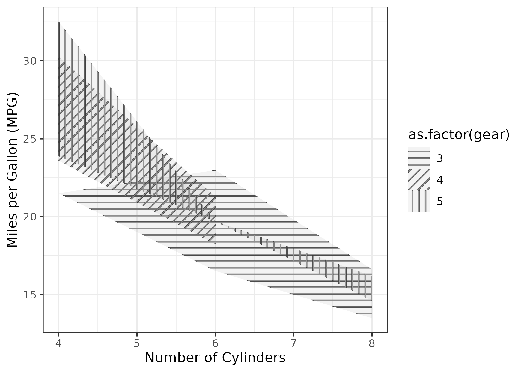
Figure 13
Keywords: step function, piece-wise constant, horizontal
library(ggplot2)
library(dplyr)

plot_df <- data.frame(x = c(-Inf, 0, 1, 2, Inf),
                      y = c(0, 1, 2, 3, 4))
text_size <- 7

gg <-
  ggplot() +
  geom_step(
    data = plot_df,
    mapping = aes(x = x,
                  y = y),
    direction = "hv",
    colour = "red",
    size = 1) +
  geom_step(
    data = plot_df,
    mapping = aes(x = x,
                  y = y),
    direction = "vh",
    colour = "blue",
    size = 1) +
  geom_point(
    data = filter(plot_df, is.finite(x)),
    mapping = aes(x = x,
                  y = y),
    size = 3) +
  geom_text(
    mapping = aes(x = 0.5,
                  y = 2.5,
                  label = "direction = \"vh\""),
    size = text_size,
    colour = "blue"
  ) +
  geom_text(
    mapping = aes(x = 1.5,
                  y = 1.5,
                  label = "direction = \"hv\""),
    size = text_size,
    colour = "red"
  ) +
  labs(
    title = "geom_step()"
  ) +
  theme_bw() +
  ## Use a fixed with font for the title text
  theme(plot.title = element_text(size = 20,
                                  family = "mono",
                                  face = "bold"))

ggsave("fig13.png",
       gg,
       height = 10.5, width = 14.8,
       units = "cm")
Figure 14
Keywords: ggpubr, significance, publication, comparison
library(ggplot2)
library(dplyr)
library(ggpubr)


my_comparisons <- list(c("setosa", "versicolor"),
                       c("setosa", "virginica"))

gg <-
  ggboxplot(data = iris,
            x = "Species",
            y = "Petal.Length",
            add = "jitter") +
  stat_compare_means(comparisons = my_comparisons,
                     label = "p.signif",
                     size = c(5, 5)) +
  scale_y_continuous(limits = c(1, 9)) +
  labs(x = NULL,
       y = "Petal length") +
  theme_bw()

ggsave("fig14.png",
       gg,
       height = 10.5, width = 14.8,
       units = "cm")
Colophon
if (!requireNamespace("BiocManager", quietly = TRUE))
  install.packages("BiocManager")

BiocManager::install("ggtree")