AANN 18/04/2026
Table of Contents
Autoencoders for computational statistics
Overview
I recently read a couple of papers from Elizaveta Semenova, PriorVAE and PriorCVAE where a decoder (from an autoencoder) is used as a surrogate in sampling from a computationally expensive Gaussian process prior. Why should you care about this? If your doing MCMC with a spatial model this can make things run much much faster.
Here we'll use MNIST digits as a substitute for real spatial data, but the idea is the same, just substitute a pixel of the image for a pixel in a map.
Background
(Variational and conditional) autoencoders
A vanilla autoencoder (neural network) is made up of two subnetworks: an encoder, which takes a high-dimensional vector \(x\) (in our example a flattened \(28\times 28\) image in \(\mathbb{R}^{784}\)) and "encodes" it in a lower-dimensional representation \(h\) (in our example \(h\in\mathbb{R}^{15}\); and a decoder, which takes that low-dimensional representation \(h\) and maps it to \(\hat{x}\), which is a reconstruction of the original high-dimensional vector \(x\). In learning how to map data into lower dimensions, and then recover it, the autoencoder learns to perform dimensionality reduction1. In Figure 1 there is an example of an autoencoder.
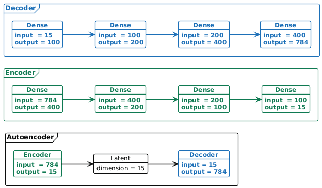
Figure 1: Example of the autoencoder architecture. Here we have an encoder (shown in detail in green in the middle) with four dense layers that map the 784 dimensional input down to 15 latent dimensions. The decoder (shown in blue in detail at the top) reconstructs the encoded data in 784 dimensions. The full network combining the encoder and decoder is shown at the bottom.
In a variational autoencoder (VAE), the lower dimensional representation is a distribution (typically a Gaussian distribution). I.e. the encoder maps \(x\) to \((\boldsymbol{\mu},\boldsymbol{\sigma}^{2})\) (the parameters of a multivariate Gaussian distribution), then the decoder takes a sample from that distribution, \(z\sim\text{N}(\boldsymbol{\mu},\boldsymbol{\sigma}^{2})\), and maps it to a reconstruction \(\hat{x}\)2. As we will see below, the loss function for training a VAE tries to keep this latent Gaussian distribution as close to a standard normal as possible. In Figure 2 there is an example of the VAE architecture.
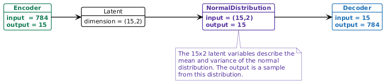
Figure 2: Example of the variational autoencoder architecture. In the purple NormalDistribution node, we sample a random vector from the normal distribution to pass to the decoder. Both the encoder and decoder are the same as they were in Figure 1.
In a conditional VAE we assume that there is some additional conditioning information \(c\) associated with each datum \(x\). In this case, the decoder takes the (concatenated) vector \((z,c)\) and maps it to the reconstruction \(\hat{x}\). In our example \(c\in\mathbb{R}^{10}\) because it is a one-hot-encoding of the digit.
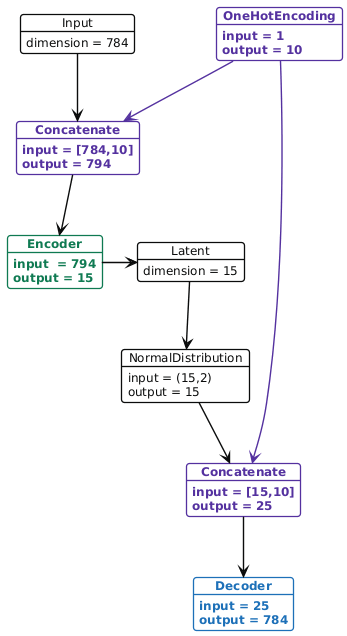
Figure 3: Example of the conditional variational autoencoder architecture. Note that in the conditional version, we concatenate (shown in purple) a one-hot-encoding of the class label (or a generic context vector) to the sample before it enters the encoder and again to the latent vector before it is decoded. Both the encoder and decoder are the same as they were in Figure 1, although the input dimensionality of the first layer in the encoder and decoder have been increased by 10 to account for the one-hot-encoding of the digit.
Loss function
There are two terms in the loss function for training a VAE: the reconstruction loss, which measures the error in the reconstruction \(\hat{x}\) of the truth \(x\), in our example I use the binary cross entropy; and the regularization loss, which measures how far the latent distribution is from a standard normal, in this example I use the Kullback-Leibler divergence (which can be computed in closed form between Gaussian distributions).
Implementation
There is an implementation of the (C)VAE and the binary cross entropy loss function here.
Example
Looking at the data
Training a VAE on 5s
I trained the VAE shown in Figure 2 to sample novel instances of the digit 5. The training process is pretty straight forward so you might be best off just looking at the script implementing it, and the script that samples from the trained model. Some samples from the trained model are shown in Figure 5.
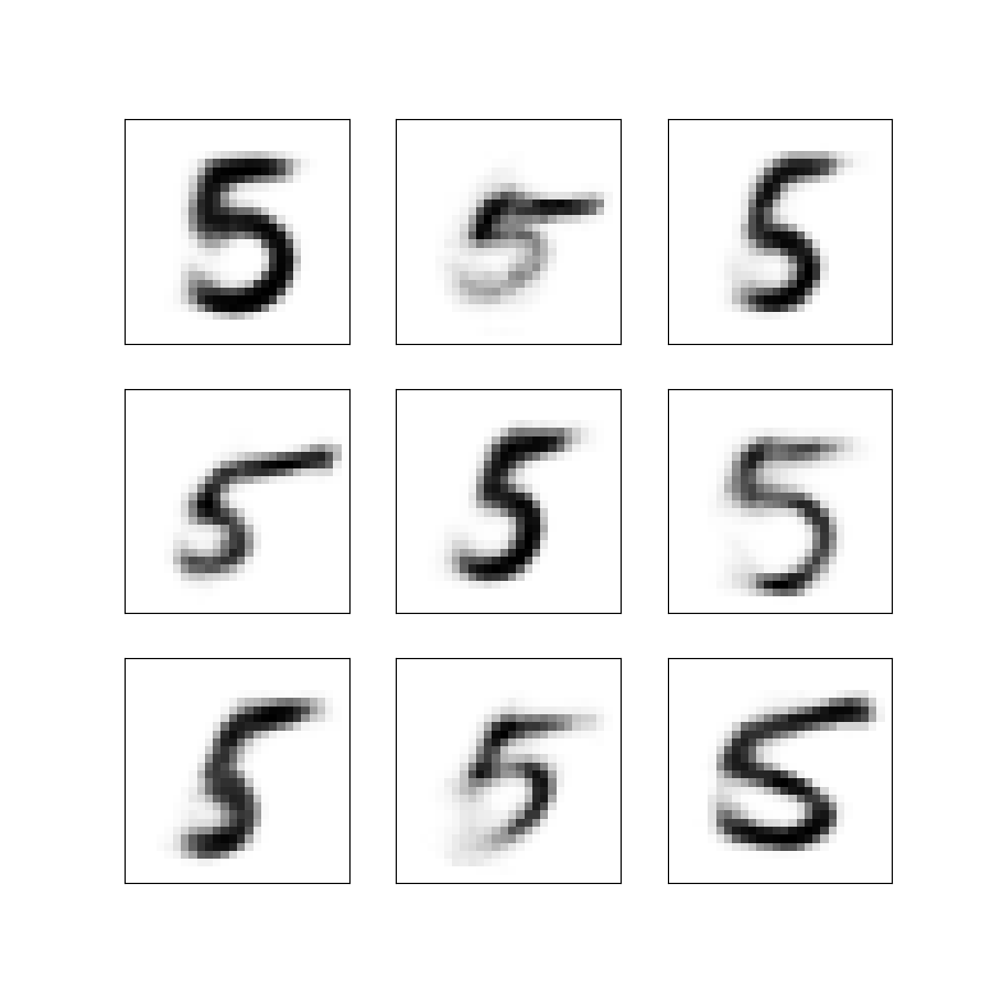
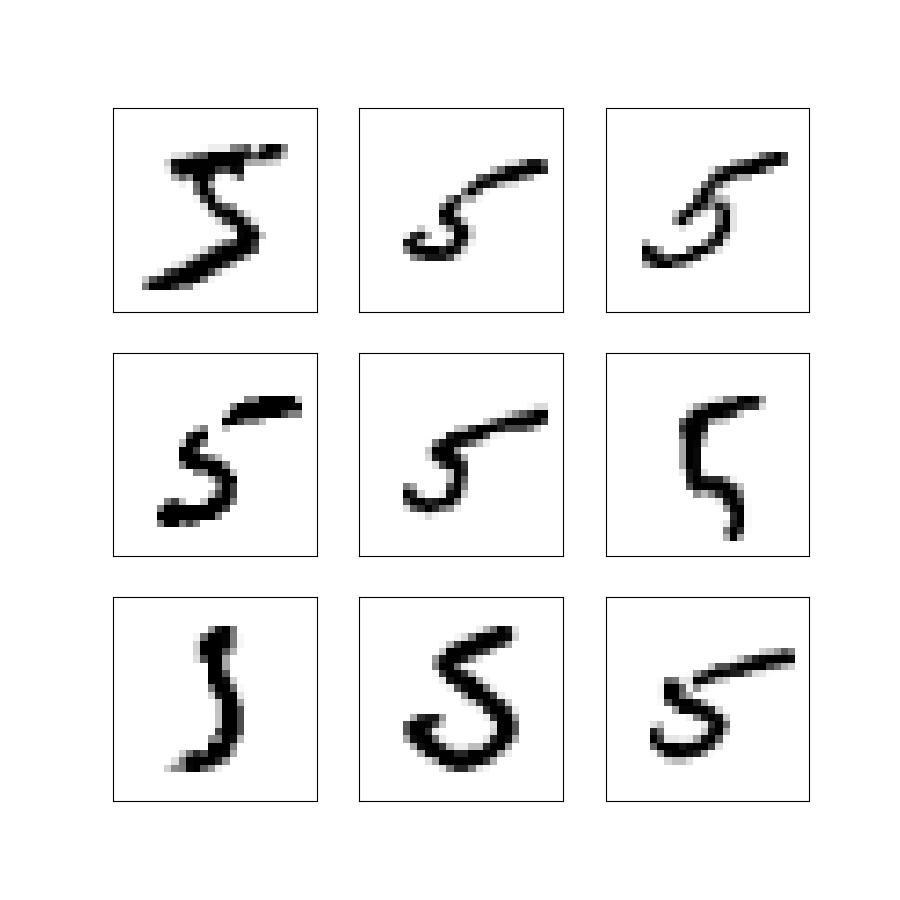
Figure 5: Nine synthetic images obtained by sampling from the latent Gaussian distribution and decoding the sample into an image.
Note that these images are not part of the training data. We have sampled new latent vectors from the standard normal distribution and used these as input to the decoder to get the images. Using the standard normal as our source of random variables is why it is important to have the KL-divergence term in the loss function.
Exploring generalization
If you were to use one of these trained decoders as a way to sample from your prior distribution, as in PriorVAE and PriorCVAE you'd want to have some confidence the decoder behaves sensibly across the region of parameter space the MCMC is likely to visit. To test this, I sampled random directions and then looked at the images generated as you moved in that direction (i.e. scaled a random vector by a factor of 0, 2 and 4). In Figure 6, examples of the generated images are shown, while the images degrade slightly, the digits are still vaguely five shaped.
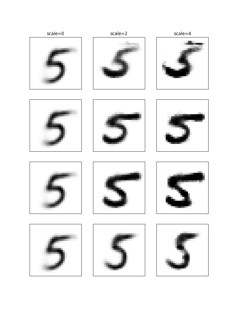
Figure 6: Images taking increasingly extreme values of the latent space
Training a conditional VAE on all the digits
I trained the CVAE shown in Figure 3 to sample novel instances of all of the digits. Again, the training process is straight forward so you might be best off just looking at the script implementing it, and the script that samples from the trained model. Some samples from the trained model are shown in Figure 7. I suspect you could get a better image if you optimised the training, but since this is only a proof of principle I won't bother; they are mostly recognisable…
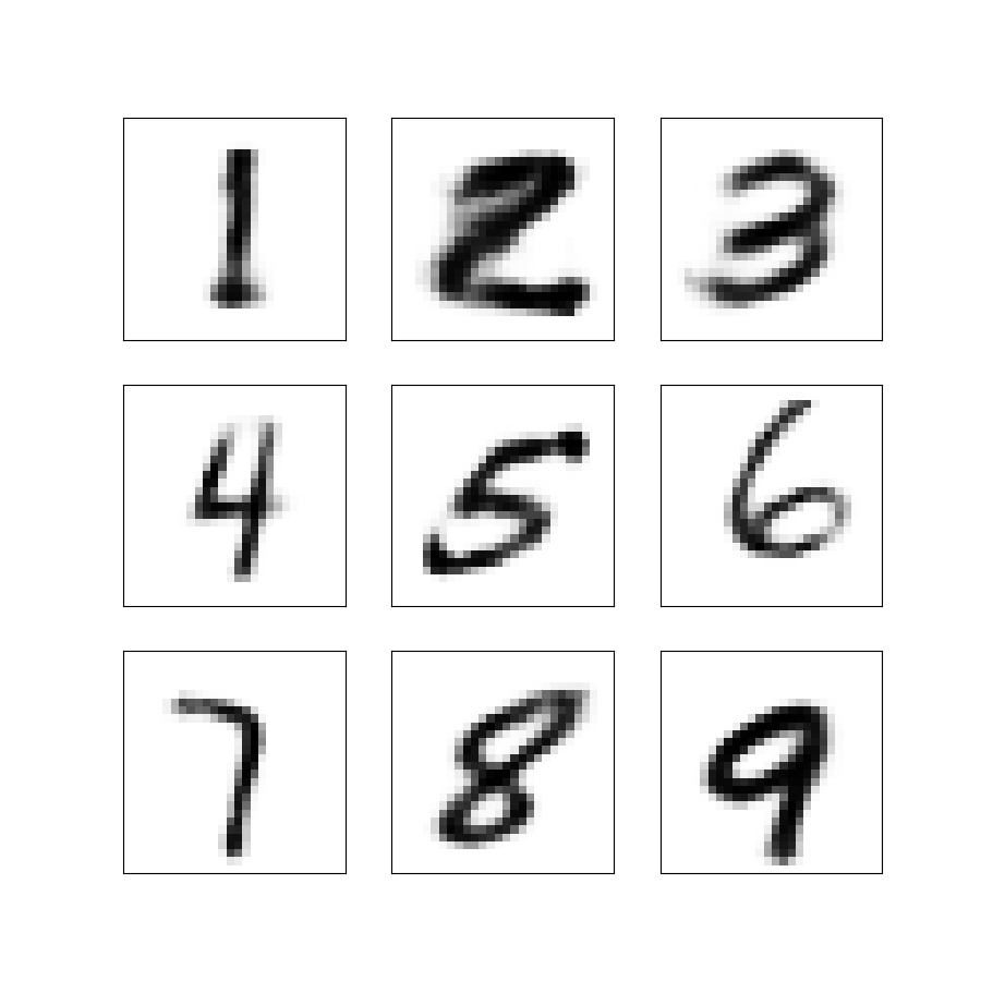
Figure 7: Nine synthetic images of the digits 1–9 obtained by sampling from the latent Gaussian distribution and decoding the sample into an image.
Use as a prior in MCMC
To get an idea for how the CVAE decoder works as a prior distribution within MCMC, we can consider the case where we start with a partial observation of a number and want to estimate what the rest of it looked like (and what number it is!) If you were applying this in the context of spatial epidemiology, this might correspond to estimating the prevalence of disease across a large area when you only have prevalence data from a few sites.
We start by taking one of MNIST digits (from the testing set), and generating a random mask of pixels to observe. In Figure 8 (left) there is a masked number three. We then set up our NumPyro model of this process of masking and observation with noise. A probabilistic program for this might look like the following:
- \(\theta\sim\text{N}_{25}(0,1)\)
- \(z\leftarrow\theta[\texttt{1:15}]\)
- \(c\leftarrow\text{softmax}(\theta[\texttt{16:25}])\)
- \(\mu_Y\leftarrow\text{Decoder}(z,c)\)
- \(Y[\texttt{mask}]\sim\text{N}(\mu_Y[\texttt{mask}], {0.1}^2)\)
With this program, we can sample from the posterior distribution and use the mean of the samples to understand what the digit is likely to be. In Figure 8 (right) there is an image of the posterior mean of the digit. The code for this is available here.
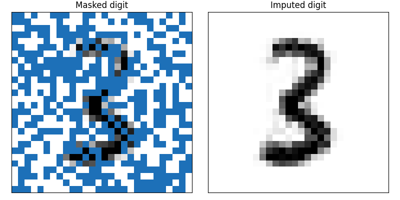
Figure 8: Using the CVAE as a prior distribution we can recover the missing pixels from a masked image. Partially masked digit given as input to the MCMC. The posterior mean of the samples for the missing pixels.
Discussion
In this post I built a (conditional) variational autoencoder to provide a mapping between the standard multivariate normal distribution and a high dimensional space of images. In this case the images are the MNIST digits, but the same idea can be applied to epidemiological maps. In fact, this approach has been used in spatial epidemiology to provide a computationally efficient way to work with Gaussian processes. Basically, you swap an array of pixels for a field that has been evaluated on a mesh, but the same idea can be applied to other kinds of complex high-dimensional prior distributions. This is a cool example of where "classical" machine learning can be applied in statistics.
Why should you care about this? If your doing MCMC with a spatial model this can make things run much much faster.
Thanks
Thank you for reading this post. Please get in touch if you have any feedback :)
Footnotes:
Dimensionality reduction is one of the main use cases for autoencoders.
In practice, this uses the reparameterization trick to avoid numerical difficulties. This is important, but perhaps less interesting.