pypfilt-notes

Pypfilt
Terminology
Examples: flipping coins
Examples: birth-death process
Colophon

Pypfilt

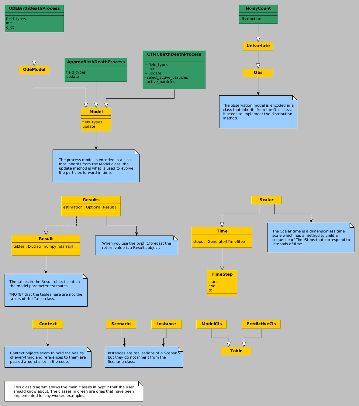
Figure 1: A class diagram showing the main classes that a user will interact with when using pypfilt along with the classes that are used in the examples on this page.

Terminology

observation model: the distribution of a random variable (e.g., the measured population size) given the state (e.g., the true population.)
process model: a stochastic process for the state, e.g., how the population size changes through time.
scenario: a description of a simulation or an inference problem, e.g., estimating the birth rate and the future population sizes. Think: "an imagined sequence of events."

Examples: flipping coins

Consider the problem of estimating the probability a coin comes up heads. Let \(\theta\) be the probability of heads. Our data are the random variables \(H_{i}|\theta\sim\text{Bernoulli}(\theta)\) for \(i=1,\ldots,5\). We will use the prior distribution \(\theta\sim\text{Beta}(1, 1)\). For \(\sum_{i=1}^{5} H_{i} = 3\), the posterior distribution is \(\theta|\mathcal{D}\sim\text{Beta}(4,3)\).

A comparison of the credible intervals for the analytic solution and the result from using a particle filter (with only 100 particles) is shown in the following figure.

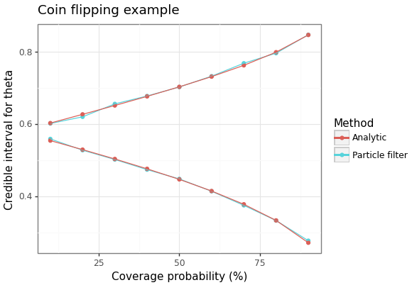
Figure 2: Credible intervals for the probability of heads based on 3 heads in 5 flips.

Data

Here is our data, saved in a file coin-results.ssv.

time value
1.0 1
2.0 0
3.0 1
4.0 0
5.0 1

Scenario file

Here is a scenario file describing the inference problem.

[components]
model = "coin_example.ConstantParameter"
time = "pypfilt.Scalar"
sampler = "pypfilt.sampler.LatinHypercube"
summary = "pypfilt.summary.HDF5"

[time]
start = 0.0
until = 5.0
steps_per_unit = 1
summaries_per_unit = 1

[prior]
theta = { name = "uniform", args.loc = 0.0, args.scale = 1.0 }

[observations.theta]
model = "coin_example.BernoulliObservation"
file = "coin-results.ssv"

[filter]
particles = 100
prng_seed = 1
history_window = 0
resample.threshold = 0.25

[scenario.inference]
summary.tables.model_cints.component = "pypfilt.summary.ModelCIs"
summary.tables.model_cints.credible_intervals = [ 10, 20, 30, 40, 50, 60, 70, 80, 90 ]

Main script

# coin-example.py
#
# program: Coin flipping example
#
# programmer: Alexander E. Zarebski
# date: 2023-08-28
#
# description: A simple example of parameter estimation with the fit
# method in a case where we know the solution analytically
#
#
import numpy as np
import scipy.stats
import pypfilt
import matplotlib.pyplot as plt
import matplotlib.image as mpimg
import matplotlib as matplotlib
matplotlib.use('QtAgg')
import pandas as pd
import plotnine as p9
from plotnine import *
#
#
#  ************************************************
#  *                                              *
#  * Define the simulation and observation models *
#  *                                              *
#  ************************************************
#
#
class ConstantParameter(pypfilt.model.Model):
    def field_types(self, ctx):
        return [('theta', np.dtype(float))]

    def init(self, ctx, vec):
        prior = ctx.data['prior']
        vec['theta'] = prior['theta']

    def update(self, ctx, time_step, is_forecast, prev, curr):
        curr[:] = prev[:]


class BernoulliObservation(pypfilt.obs.Univariate):
    def distribution(self, ctx, snapshot):
        p = snapshot.state_vec[self.unit]
        return scipy.stats.bernoulli(p)
#
#
#  ***************************************************
#  *                                                 *
#  * Use the particle filter to sample the posterior *
#  *                                                 *
#  ***************************************************
#
#
inst = list(pypfilt.load_instances("coin.toml"))[0]
ctx = inst.build_context()
fit = pypfilt.fit(ctx, filename=None)
pst_df = pd.DataFrame(fit.estimation.tables['model_cints'])
pst_df = pst_df[pst_df['time'] == 5.0][['prob','ymin', 'ymax']]
#
#
#  ************************************************
#  *                                              *
#  * Plot the approximate and analytic posteriors *
#  *                                              *
#  ************************************************
#
#
coin_flips = pd.read_table("coin-results.ssv", sep = ' ')['value']
num_flips = coin_flips.size
num_heads = coin_flips.sum()
post_dist = scipy.stats.beta(a = num_heads + 1, b = num_flips - num_heads + 1)

plt_df = pst_df.copy()
plt_df['ymax_beta'] = post_dist.ppf(1 - 0.01 * 0.5 * (100 - plt_df['prob']))
plt_df['ymin_beta'] = post_dist.ppf(0.01 * 0.5 * (100 - plt_df['prob']))
plt_df = pd.melt(plt_df,
                 id_vars = ['prob'],
                 value_vars = ['ymin', 'ymax', 'ymin_beta', 'ymax_beta'])
plt_df['type'] = plt_df['variable'].apply(lambda v: 'Analytic' if ('beta' in v) else 'Particle filter')

cri_p9 = (ggplot()
          + geom_point(
              data = plt_df,
              mapping = aes(x = "prob",
                            y = "value",
                            color = "type"))
          + geom_line(
              data = plt_df,
              mapping = aes(x = "prob",
                            y = "value",
                            color = "type",
                            group = "variable"))
          + labs(title = "Coin flipping example",
                 y = "Credible interval for theta",
                 x = "Coverage probability (%)",
                 color = "Method")
          + theme_bw()

    )
cri_p9.save("coin-example.png",
        height = 4.1, width = 5.8)

Examples: birth-death process

We can model the birth-death process in a number of ways:

with Tau-leaping;
with ODEs; and again using the fit method;
and as a CTMC.

For each example, we will consider observations with Poisson noise about the true state. The observation model is described with the NoisyCount observation distribution.

Observation model

As stated above, we will assume Poisson noise about the true value of the state. This is implemented as the NoisyCount class. This class will be used with each of the different process representations.

# NoisyCount.py

<<imports>>

class NoisyCount(pypfilt.obs.Univariate):
    def distribution(self, ctx, snapshot):
        expected_value = snapshot.state_vec['x']
        return scipy.stats.poisson(mu=expected_value)

Tau-leaping birth-death

Consider an approximation of the birth-death process using \(\tau\)-leaping. The following example demonstrates how to simulate from this process and run a forecast to estimate both the future state and the birth rate (assuming a known death rate and initial condition).

Process model

We start by defining a model for this process using \(\tau\)-leaping.

# TauLeapBirthDeathProcess.py

<<imports>>

class TauLeapBirthDeathProcess(pypfilt.model.Model):
    def field_types(self, ctx):
        return [('birth', np.dtype(float)),
                ('death', np.dtype(float)),
                ('x', np.dtype(int))]

    def update(self, ctx, time_step, is_fs, prev, curr):
        """Destructively update the current state."""
        rnd = ctx.component['random']['model']
        net_rate = (prev['birth'] - prev['death']) * time_step.dt * prev['x']
        curr['birth'] = prev['birth']
        curr['death'] = prev['death']
        curr['x'] = prev['x'] + rnd.poisson(lam=net_rate, size=curr['x'].shape)

Note that in the update method we need to destructively update curr to contain the new value. I.e., curr should be considered a reference to the state, this avoids needing to make a copy of this data.

Scenario file

The simulation and estimation computations are specified with a TOML file approx-bd-example.toml.

[metadata]
name = "Tau leap birth-death example"
filename = "tau-leap-bd-example.toml"
author = "Alexander E. Zarebski"
date = "2023-07-25"

[components]
model = "TauLeapBirthDeathProcess.TauLeapBirthDeathProcess"
time = "pypfilt.Scalar"
sampler = "pypfilt.sampler.LatinHypercube"
summary = "pypfilt.summary.HDF5"

[time]
start = 0.0
until = 5.0
steps_per_unit = 10
summaries_per_unit = 2

[prior]
death = { name = "constant", args.value = 1.0 }
x = { name = "constant", args.value = 1 }

[observations.x]
model = "NoisyCount.NoisyCount"
file = "tau-leap-bd-example-x.ssv"

[filter]
particles = 10000
prng_seed = 42
history_window = -1
resample.threshold = 0.25
regularisation.enabled = true

[scenario.simulate]
prior.birth = { name = "constant", args.value = 2.0 }

[scenario.forecast]
summary.tables.model_cints.component = "pypfilt.summary.ModelCIs"
summary.tables.model_cints.credible_intervals = [ 0, 25, 50, 75, 95 ]
summary.tables.forecasts.component = "pypfilt.summary.PredictiveCIs"
summary.tables.forecasts.credible_intervals = [10, 20, 40, 80]
prior.birth = { name = "uniform", args.loc = 1.0, args.scale = 3.0 }
backcast_time = 0.0
forecast_time = 4.0

[output]
credible_intervals = "demo-tau-leap-bd-cris.ssv"
estimate_plot = "tau-leap-bd-posterior-estimates.png"
forecast_plot = "tau-leap-bd-posterior-forecasts.png"

Note, apart from scenario.simulate and scenario.forecast, all the configuration is shared between the two tasks. The process model and observation model needs to be described with both the module and the class within it.

The specification of the prior distributions appears to take the location as the right end of the uniform distribution and the scale is the width of the uniform distribution. This may not be wildly intuitive, but bear in mind that there are sophisticated options for specifying a prior distribution available.

Main script

Here is the main script that runs the simulation and estimation.

# tau-leap-bd-example.py

<<imports>>
<<plotting-imports>>

scenario_file = 'tau-leap-bd-example.toml'
instances = list(pypfilt.load_instances(scenario_file))
sim_instance = instances[0]
my_time_scale = sim_instance.time_scale()
my_obs_tables = pypfilt.simulate_from_model(sim_instance)

for (obs_unit, obs_table) in my_obs_tables.items():
    out_file = f'tau-leap-bd-example-{obs_unit}.ssv'
    pypfilt.io.write_table(out_file, obs_table, my_time_scale)

To run the forecasts on the simulated data we have the following

fst_instance = instances[1]
backcast_time = fst_instance.settings['backcast_time']
forecast_time = fst_instance.settings['forecast_time']
context = fst_instance.build_context()
results = pypfilt.forecast(context, [forecast_time], filename=None)

We can generate a plot of the forecast values, and the estimate of the historical states of the process.

fit = results.estimation.tables['forecasts']
forecast = results.forecasts[forecast_time].tables['forecasts']
credible_intervals = np.concatenate((
    fit[fit['time'] >= backcast_time],
    forecast))

cri_df = pd.DataFrame(credible_intervals)
cri_df = cri_df.assign(prob = cri_df['prob'])
obs_df = pd.read_csv('tau-leap-bd-example-x.ssv', sep=' ')
obs_df = obs_df[obs_df['time'] >= backcast_time]
obs_df = obs_df.assign(observed = obs_df['time'] <= forecast_time)

fs_p9 = (ggplot()
         + geom_ribbon(data = cri_df,
                       mapping = aes(x = "time",
                                     ymin = "ymin",
                                     ymax = "ymax",
                                     group = "prob"),
                       alpha = 0.2)
         + scale_x_continuous(name = "Time")
         + scale_y_sqrt(name = "Population size")
         + geom_point(data = obs_df,
                      mapping = aes(x = "time",
                                    y = "value",
                                    shape = "observed"),
                      size = 3,
                      colour = "red")
         + scale_shape_manual(values = {True: 'o', False: 'x'})
         + geom_vline(xintercept = forecast_time,
                      linetype = "dashed")
         + labs(title = "Population size forecast")
         + theme_bw()
         + theme(legend_position = "none"))

fs_p9.save(instances[1].settings['output']['forecast_plot'],
           height = 4.1, width = 5.8)

Here are the results of the particle filter.

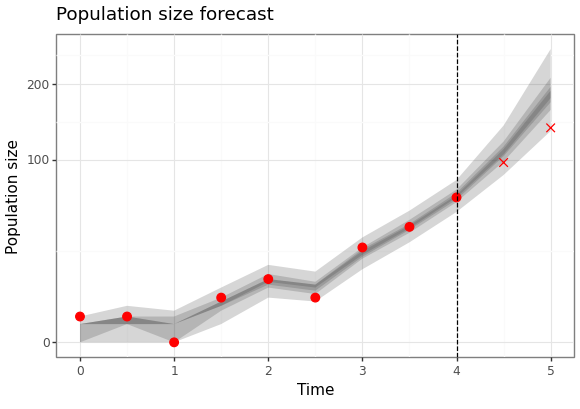
Figure 3: Forecast of birth-death process

We can also generate a plot of how the posterior distribution converges on the true value of the parameter as the amount of data available increases.

param_cris_df = pd.DataFrame(results.estimation.tables['model_cints'])
param_cris_df = param_cris_df[param_cris_df['name'] == 'birth']
param_cris_df['prob'] = pd.Categorical(
    param_cris_df['prob'],
    categories=param_cris_df['prob'].unique(),
    ordered=True
)
pt_est_mask = param_cris_df['prob'] == 0

br_p9 = (ggplot()
         + geom_ribbon(data = param_cris_df,
                       mapping = aes(x = "time",
                                     ymin = "ymin",
                                     ymax = "ymax",
                                     group = "prob"),
                       alpha = 0.2,
                       size = 1)
         + geom_line(data = param_cris_df[pt_est_mask],
                     mapping = aes(x = "time",
                                   y = "ymin"))
         + geom_hline(yintercept = 2.0, linetype = "dashed", colour = "red")
         + scale_x_continuous(name = "Amount of data used")
         + scale_y_continuous(name = "Birth rate")
         + labs(title = "Birth rate credible intervals")
         + theme_bw())

br_p9.save(instances[1].settings['output']['estimate_plot'],
           height = 4.1, width = 5.8)

Here are the results of the particle filter.

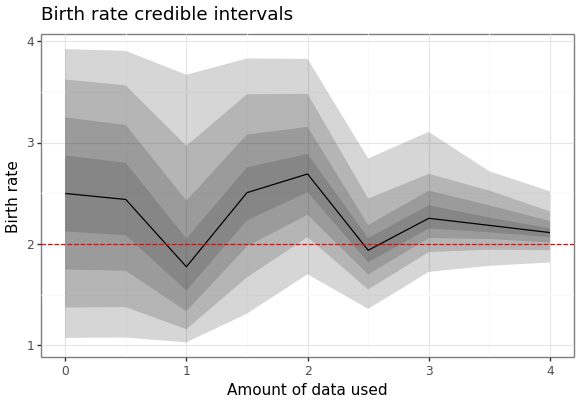
Figure 4: Forecast of birth-death process

ODE birth-death

Consider an approximation of the birth-death process using a differential equation.

Process model

We start by defining a model for this process which is adapted from this example.

# ODEBirthDeathProcess.py

<<imports>>

class ODEBirthDeathProcess(pypfilt.model.OdeModel):
    def field_types(self, ctx):
        return [('birth', np.dtype(float)),
                ('death', np.dtype(float)),
                ('x', np.dtype(float))]

    def init(self, ctx, vec):
        prior = ctx.data['prior']
        vec['x'] = prior['x']
        vec['birth'] = prior['birth']
        vec['death'] = prior['death']
        self.method = 'RK45'

    def d_dt(self, time, xt, ctx, is_forecast):
        d_dt = np.zeros(xt.shape, dtype=xt.dtype)
        d_dt['x'] = (xt['birth'] - xt['death']) * xt['x']
        return d_dt

Scenario file

The simulation and estimation computations are specified with a TOML file ode-bd-example.toml.

[metadata]
name = "ODE birth-death example"
filename = "ode-bd-example.toml"
author = "Alexander E. Zarebski"
date = "2023-07-27"

[components]
model = "ODEBirthDeathProcess.ODEBirthDeathProcess"
time = "pypfilt.Scalar"
sampler = "pypfilt.sampler.LatinHypercube"
summary = "pypfilt.summary.HDF5"

[time]
start = 0.0
until = 5.0
steps_per_unit = 10
summaries_per_unit = 2

[prior]
death = { name = "constant", args.value = 1.0 }
x = { name = "constant", args.value = 1 }

[observations.x]
model = "NoisyCount.NoisyCount"
file = "ode-bd-example-x.ssv"

[filter]
particles = 10000
prng_seed = 13
history_window = -1
resample.threshold = 0.25
regularisation.enabled = true

[scenario.simulate]
prior.birth = { name = "constant", args.value = 2.0 }

[scenario.forecast]
summary.tables.model_cints.component = "pypfilt.summary.ModelCIs"
summary.tables.model_cints.credible_intervals = [ 0, 25, 50, 75, 95 ]
summary.tables.forecasts.component = "pypfilt.summary.PredictiveCIs"
summary.tables.forecasts.credible_intervals = [10, 20, 40, 80]
prior.birth = { name = "uniform", args.loc = 1.75, args.scale = 0.5 }
backcast_time = 2.0
forecast_time = 4.0

[output]
credible_intervals = "demo-ode-bd-cris.ssv"
estimate_plot = "ode-bd-posterior-estimates.png"
forecast_plot = "ode-bd-posterior-forecasts.png"

Main script

Here is the main script that runs the simulation and estimation.

# ode-bd-example.py

<<imports>>
<<plotting-imports>>

scenario_file = 'ode-bd-example.toml'
instances = list(pypfilt.load_instances(scenario_file))
sim_instance = instances[0]
my_time_scale = sim_instance.time_scale()
my_obs_tables = pypfilt.simulate_from_model(sim_instance)

for (obs_unit, obs_table) in my_obs_tables.items():
    out_file = f'ode-bd-example-{obs_unit}.ssv'
    pypfilt.io.write_table(out_file, obs_table, my_time_scale)

To run the forecasts on the simulated data we have the following

fst_instance = instances[1]
backcast_time = fst_instance.settings['backcast_time']
forecast_time = fst_instance.settings['forecast_time']
context = fst_instance.build_context()
results = pypfilt.forecast(context, [forecast_time], filename=None)

Then finally we can generate a plot showing both the future forecasted values, but also the estiamte of the historical states of the process.

fit = results.estimation.tables['forecasts']
forecast = results.forecasts[forecast_time].tables['forecasts']
credible_intervals = np.concatenate((
    fit[fit['time'] >= backcast_time],
    forecast))

cri_df = pd.DataFrame(credible_intervals)
cri_df = cri_df.assign(prob = cri_df['prob'])
obs_df = pd.read_csv('ode-bd-example-x.ssv', sep=' ')
obs_df = obs_df[obs_df['time'] >= backcast_time]
obs_df = obs_df.assign(observed = obs_df['time'] <= forecast_time)

fs_p9 = (ggplot()
         + geom_ribbon(data = cri_df,
                       mapping = aes(x = "time",
                                     ymin = "ymin",
                                     ymax = "ymax",
                                     group = "prob",
                                     fill = "prob"),
                       alpha = 0.5)
         + scale_fill_gradient(low = "white", high = "black")
         + scale_x_continuous(name = "Time")
         + scale_y_continuous(name = "Population size")
         + geom_point(data = obs_df,
                      color = "red",
                      mapping = aes(x = "time",
                                    y = "value",
                                    shape = "observed"),
                      size = 3)
         + scale_shape_manual(values = {True: 'o', False: 'x'})
         + geom_vline(xintercept = forecast_time,
                      linetype = "dashed")
         + labs(title = "Population size forecast")
         + theme_bw()
         + theme(legend_position = "none"))

png_plot_fn = instances[1].settings['output']['forecast_plot']
pdf_plot_fn = png_plot_fn.replace("png", "pdf")
p9.save_as_pdf_pages([fs_p9], filename = pdf_plot_fn)
import os
os.system(f"convert -density 300 {pdf_plot_fn} {png_plot_fn}")
os.remove(pdf_plot_fn)

Here are the results of the particle filter (with the code to create the figure below).

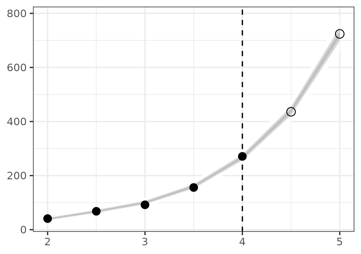
Figure 5: Forecast of birth-death process

We can also generate a plot of how the posterior distribution converges on the true value of the parameter as the amount of data available increases.

param_cris_df = pd.DataFrame(results.estimation.tables['model_cints'])
param_cris_df = param_cris_df[param_cris_df['name'] == 'birth']
param_cris_df['prob'] = pd.Categorical(
    param_cris_df['prob'],
    categories=param_cris_df['prob'].unique(),
    ordered=True
)
pt_est_mask = param_cris_df['prob'] == 0

br_ests_p9 = (ggplot()
              + geom_ribbon(data = param_cris_df,
                            mapping = aes(x = "time",
                                          ymin = "ymin",
                                          ymax = "ymax",
                                          group = "prob"),
                            alpha = 0.2,
                            size = 1)
              + geom_line(data = param_cris_df[pt_est_mask],
                          mapping = aes(x = "time",
                                        y = "ymin"))
              + geom_hline(yintercept = 2.0, linetype = "dashed")
              + scale_x_continuous(name = "Amount of data used")
              + scale_y_continuous(name = "Birth rate")
              + labs(title = "Birth rate credible intervals")
              + theme_bw())

png_plot_fn = instances[1].settings['output']['estimate_plot']
pdf_plot_fn = png_plot_fn.replace("png", "pdf")
p9.save_as_pdf_pages([br_ests_p9], filename = pdf_plot_fn)
import os
os.system(f"convert -density 300 {pdf_plot_fn} {png_plot_fn}")
os.remove(pdf_plot_fn)

Here are the results of the particle filter.

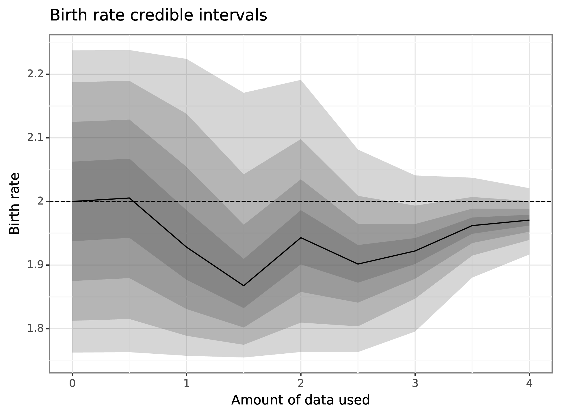
Figure 6: Forecast of birth-death process

ODE birth-death (again)

We will now use the ODE model (from before), but this time instead of using the forecast method from pypfilt we will use the fit one.

For the process model, we will use the same one as before.

Scenario file

[metadata]
name = "ODE birth-death example (again)"
filename = "ode-bd-again-example.toml"
author = "Alexander E. Zarebski"
date = "2023-09-15"

[components]
model = "ODEBirthDeathProcess.ODEBirthDeathProcess"
time = "pypfilt.Scalar"
sampler = "pypfilt.sampler.LatinHypercube"
summary = "pypfilt.summary.HDF5"

[summary.monitors]
backcast_monitor.component = "pypfilt.summary.BackcastMonitor"
backcast_monitor.foo = "bar"

[summary.tables]
backcasts.component = "BackcastStateCIs.BackcastStateCIs"
backcasts.backcast_monitor = "backcast_monitor"
backcasts.credible_intervals = [ 0, 25, 50, 75, 95 ]

[time]
start = 0.0
until = 5.0
steps_per_unit = 10
summaries_per_unit = 2

[prior]
death = { name = "constant", args.value = 1.0 }
x = { name = "constant", args.value = 1 }
birth = { name = "uniform", args.loc = 1.75, args.scale = 0.5 }

# We will re-use the simulated data set from the last example.
[observations.x]
model = "NoisyCount.NoisyCount"
file = "ode-bd-example-x.ssv"

[filter]
particles = 10000
prng_seed = 13
history_window = -1
resample.threshold = 0.25
regularisation.enabled = true

[scenario.fit]
summary.tables.model_cints.component = "pypfilt.summary.ModelCIs"
summary.tables.model_cints.credible_intervals = [ 0, 25, 50, 75, 95 ]

[output]
estimate_plot = "ode-bd-again-posterior-birth-rate-estimates.png"
state_plot = "ode-bd-posterior-state-estimates.png"

Backcast table component

We need to make a small adjustment to specify the way in which the backcast should be generated (since we are using fit instead of forecast).

# BackcastState.py

import pypfilt

class BackcastStateCIs(pypfilt.summary.BackcastPredictiveCIs):
    def n_rows(self, ctx, forecasting):
        n_obs_models = len(ctx.component['obs'])
        n_backcast_times = ctx.summary_count()
        return len(self._BackcastPredictiveCIs__probs) * n_backcast_times * n_obs_models

Main script

# ode-bd-again-example.py

<<imports>>
<<plotting-imports>>

scenario_file = "ode-bd-again-example.toml"

fit_inst = list(pypfilt.load_instances(scenario_file))[0]

context = fit_inst.build_context()

results = pypfilt.fit(context, filename=None)

Using the backcasts, see the smoothed estimates of the state in the past.

data_df = pd.read_csv(context.settings['observations']['x']['file'],
                      sep = ' ')

bc_df = pd.DataFrame(results.estimation.tables['backcasts'])
pt_est_mask = bc_df['prob'] == 0

bc_p9 = (ggplot()
         + geom_ribbon(data = bc_df,
                       mapping = aes(x = "time",
                                     ymin = "ymin",
                                     ymax = "ymax",
                                     group = "prob"),
                       alpha = 0.2,
                       size = 1)
         + geom_line(data = bc_df[pt_est_mask],
                     mapping = aes(x = "time",
                                   y = "ymin"))
         + geom_point(data = data_df,
                      mapping = aes(x = "time", y = "value"))
         + scale_y_log10(name = "")
         + scale_x_continuous(name = "")
         + labs(title = "State credible intervals")
         + theme_bw())

bc_p9.save(context.settings['output']['state_plot'],
        height = 5.8, width = 8.3)

Use a ribbon plot to see how the uncertainty in the parameter estimates chnages over time.

param_cris_df = pd.DataFrame(results.estimation.tables['model_cints'])
param_cris_df = param_cris_df[param_cris_df['name'] == 'birth']
param_cris_df['prob'] = pd.Categorical(
    param_cris_df['prob'],
    categories=param_cris_df['prob'].unique(),
    ordered=True
)
pt_est_mask = param_cris_df['prob'] == 0

br_ests_p9 = (ggplot()
              + geom_ribbon(data = param_cris_df,
                            mapping = aes(x = "time",
                                          ymin = "ymin",
                                          ymax = "ymax",
                                          group = "prob"),
                            alpha = 0.2,
                            size = 1)
              + geom_line(data = param_cris_df[pt_est_mask],
                          mapping = aes(x = "time",
                                        y = "ymin"))
              + geom_hline(yintercept = 2.0, linetype = "dashed")
              + scale_x_continuous(name = "Amount of data used")
              + scale_y_continuous(name = "Birth rate")
              + labs(title = "Birth rate credible intervals")
              + theme_bw())

br_ests_p9.save(context.settings['output']['estimate_plot'],
                height = 5.8, width = 8.3)

What if I want the actual trajectories?

context = fit_inst.build_context()
results = pypfilt.fit(context, filename=None)

In order to estimate the historical state of the process we need to resample the particles so they form a uniformly weighted sample and then create a "backcast" using these. When resampling, we take the last slice which correspnds to the particles at the end of the history window.

pypfilt.resample.resample(context,
                          results.estimation.history.matrix[-1, :])
my_backcast = results.estimation.history.create_backcast(context)
assert np.unique(my_backcast.matrix['weight']).shape == (1,)

Reading the backcast into a data frame for plotting is complicated by there being multiple dimensions so we reshape it first into a suitable form.

bc_df = np.reshape(my_backcast.matrix['state_vec'], -1)
bc_df = pd.DataFrame(bc_df)
bc_df['time'] = np.repeat(my_backcast.times, context.particle_count())

CTMC birth-death

Consider the birth-death process modelled with a CTMC.

Process model

We start by defining a model for this process which is adapted from this example.

# CTMCBirthDeathProcess.py

<<imports>>

class CTMCBirthDeathProcess(pypfilt.model.Model):
    def field_types(self, ctx):
        return [('birth', np.dtype(float)),
                ('death', np.dtype(float)),
                ('x', np.dtype(int)),
                ('next_event', np.int_),
                ('next_time', np.float_)]

    def init(self, ctx, vec):
        prior = ctx.data['prior']
        vec['x'] = prior['x']
        vec['birth'] = prior['birth']
        vec['death'] = prior['death']
        vec['next_time'] = 0
        vec['next_event'] = 0
        self.select_next_event(ctx, vec, stop_time=0)

    def update(self, ctx, time_step, is_forecast, prev, curr):
        curr[:] = prev[:]
        active = self.active_particles(curr, time_step.end)
        while any(active):
            births = np.logical_and(active, curr['next_event'] == 0)
            curr['x'][births] += 1
            deaths = np.logical_and(active, curr['next_event'] == 1)
            curr['x'][deaths] -= 1
            self.select_next_event(ctx, curr, stop_time=time_step.end)
            active = self.active_particles(curr, time_step.end)

    def active_particles(self, vec, stop_time):
        return np.logical_and(
            vec['next_time'] <= stop_time,
            vec['x'] > 0,
        )

    def select_next_event(self, ctx, vec, stop_time):
        active = self.active_particles(vec, stop_time)
        if not any(active):
            return

        x = vec['x'][active]
        birth = vec['birth'][active]
        death = vec['death'][active]

        birth_rate = birth * x
        death_rate = death * x
        rate_sum = birth_rate + death_rate

        rng = ctx.component['random']['model']
        dt = - np.log(rng.random(x.shape)) / rate_sum
        vec['next_time'][active] += dt

        threshold = rng.random(x.shape) * rate_sum
        death_event = threshold > birth_rate
        vec['next_event'][active] = death_event.astype(np.int_)

    def can_smooth(self):
        return {'birth'}

Scenario file

The simulation and estimation computations are specified with a TOML file ctmc-bd-example.toml.

[metadata]
name = "CTMC birth-death example"
filename = "ctmc-bd-example.toml"
author = "Alexander E. Zarebski"
date = "2023-07-27"

[components]
model = "CTMCBirthDeathProcess.CTMCBirthDeathProcess"
time = "pypfilt.Scalar"
sampler = "pypfilt.sampler.LatinHypercube"
summary = "pypfilt.summary.HDF5"

[time]
start = 0.0
until = 5.0
steps_per_unit = 10
summaries_per_unit = 2

[prior]
death = { name = "constant", args.value = 1.0 }
x = { name = "constant", args.value = 1 }

[observations.x]
model = "NoisyCount.NoisyCount"
file = "ctmc-bd-example-x.ssv"

[filter]
particles = 1000
prng_seed = 1
history_window = -1
resample.threshold = 0.25
regularisation.enabled = true

[filter.regularisation.bounds]
birth = { min = 1.0, max = 3.0 }

[scenario.simulate]
prior.birth = { name = "constant", args.value = 2.0 }

[scenario.forecast]
summary.tables.model_cints.component = "pypfilt.summary.ModelCIs"
summary.tables.model_cints.credible_intervals = [ 0, 25, 50, 75, 95 ]
summary.tables.forecasts.component = "pypfilt.summary.PredictiveCIs"
summary.tables.forecasts.credible_intervals = [10, 20, 40, 80]
prior.birth = { name = "uniform", args.loc = 1.0, args.scale = 3.0 }
backcast_time = 0.0
forecast_time = 4.0

[output]
estimate_plot = "ctmc-bd-posterior-estimates.png"
forecast_plot = "ctmc-bd-posterior-forecasts.png"

Main script

Here is the main script that runs the simulation and estimation. Because there is a substantial chance of the process going extinct, we wrap the simulation in a loop, incrementing the seed until we find one that gives an interesting simulation.

# ctmc-bd-example.py

<<imports>>
<<plotting-imports>>

scenario_file = 'ctmc-bd-example.toml'
found_good_seed=False
seed = 0
while not found_good_seed:
    print("Trying seed", seed)
    instances = list(pypfilt.load_instances(scenario_file))
    sim_instance = instances[0]
    sim_instance.settings['filter']['prng_seed'] = seed
    my_time_scale = sim_instance.time_scale()
    my_obs_tables = pypfilt.simulate_from_model(sim_instance)
    found_good_seed = my_obs_tables['x']['value'][-1] > 0
    seed += 1

for (obs_unit, obs_table) in my_obs_tables.items():
    out_file = f'ctmc-bd-example-{obs_unit}.ssv'
    pypfilt.io.write_table(out_file, obs_table, my_time_scale)

To run the forecasts on the simulated data we have the following

fst_instance = instances[1]
backcast_time = fst_instance.settings['backcast_time']
forecast_time = fst_instance.settings['forecast_time']
context = fst_instance.build_context()
results = pypfilt.forecast(context, [forecast_time], filename=None)

Then finally we can generate a plot showing both the future forecasted values, but also the estiamte of the historical states of the process.

fit = results.estimation.tables['forecasts']
forecast = results.forecasts[forecast_time].tables['forecasts']
credible_intervals = np.concatenate((
    fit[fit['time'] >= backcast_time],
    forecast))

cri_df = pd.DataFrame(credible_intervals)
cri_df = cri_df.assign(prob = cri_df['prob'])
obs_df = pd.read_csv('ctmc-bd-example-x.ssv', sep=' ')
obs_df = obs_df[obs_df['time'] >= backcast_time]
obs_df = obs_df.assign(observed = obs_df['time'] <= forecast_time)

fs_p9 = (ggplot()
         + geom_ribbon(data = cri_df,
                       mapping = aes(x = "time",
                                     ymin = "ymin",
                                     ymax = "ymax",
                                     group = "prob"),
                       alpha = 0.2)
         + scale_x_continuous(name = "Time")
         + scale_y_sqrt(name = "Population size")
         + geom_point(data = obs_df,
                      mapping = aes(x = "time",
                                    y = "value",
                                    shape = "observed"),
                      size = 3,
                      colour = "red")
         + scale_shape_manual(values = {True: 'o', False: 'x'})
         + geom_vline(xintercept = forecast_time,
                      linetype = "dashed")
         + labs(title = "Population size forecast")
         + theme_bw()
         + theme(legend_position = "none"))

fs_p9.save(instances[1].settings['output']['forecast_plot'],
           height = 4.1, width = 5.8)

Here are the results of the particle filter (with the code to create the figure below).

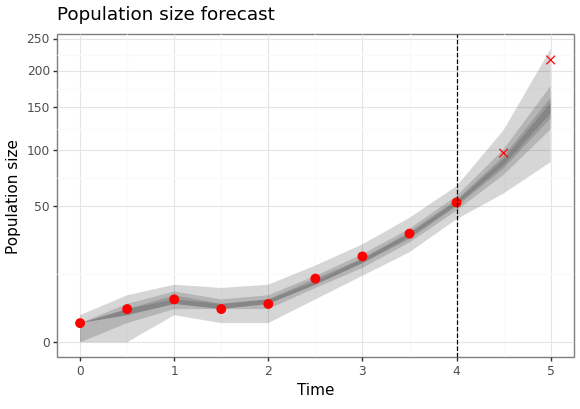
Figure 7: Forecast of birth-death process

We can also generate a plot of how the posterior distribution converges on the true value of the parameter as the amount of data available increases.

param_cris_df = pd.DataFrame(results.estimation.tables['model_cints'])
param_cris_df = param_cris_df[param_cris_df['name'] == 'birth']
param_cris_df['prob'] = pd.Categorical(
    param_cris_df['prob'],
    categories=param_cris_df['prob'].unique(),
    ordered=True
)
pt_est_mask = param_cris_df['prob'] == 0

br_p9 = (ggplot()
         + geom_ribbon(data = param_cris_df,
                       mapping = aes(x = "time",
                                     ymin = "ymin",
                                     ymax = "ymax",
                                     group = "prob"),
                       alpha = 0.2,
                       size = 1)
         + geom_line(data = param_cris_df[pt_est_mask],
                     mapping = aes(x = "time",
                                   y = "ymin"))
         + geom_hline(yintercept = 2.0, linetype = "dashed", colour = "red")
         + scale_x_continuous(name = "Amount of data used")
         + scale_y_continuous(name = "Birth rate")
         + labs(title = "Birth rate credible intervals")
         + theme_bw())

br_p9.save(instances[1].settings['output']['estimate_plot'],
           height = 4.1, width = 5.8)

Here are the results of the particle filter.

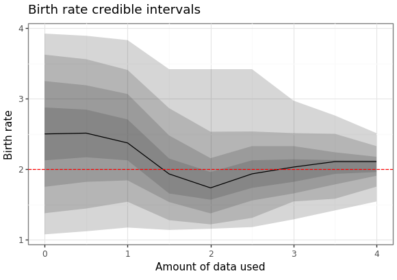
Figure 8: Forecast of birth-death process

Colophon

Here is a requirements file for a python virtual environment to run these examples.

contourpy==1.1.0
cycler==0.11.0
fonttools==4.41.1
h5py==3.9.0
kiwisolver==1.4.4
lhs==0.4.1
matplotlib==3.7.2
mizani==0.9.2
numpy==1.25.1
packaging==23.1
pandas==2.0.3
patsy==0.5.3
Pillow==10.0.0
plotnine==0.12.2
pyparsing==3.0.9
pypfilt==0.8.0
PyQt5==5.15.9
PyQt5-Qt5==5.15.2
PyQt5-sip==12.12.2
python-dateutil==2.8.2
pytz==2023.3
scipy==1.11.1
six==1.16.0
statsmodels==0.14.0
tomli==2.0.1
tomli_w==1.0.0
tzdata==2023.3

Once you have the virtual environment set up, the examples can be run as shown in the following example when using the \(\tau\)-leaping code.

$ python tau-leap-bd-example.py

Here is a source block that gets included whenever you see an imports statement.

import numpy as np
import scipy.stats
import pypfilt

import matplotlib.pyplot as plt
import matplotlib.image as mpimg
import matplotlib as matplotlib
matplotlib.use('QtAgg')
import pandas as pd
import plotnine as p9
from plotnine import *

pypfilt-notes

Table of Contents

Pypfilt

Terminology

Examples: flipping coins

Data

Scenario file

Main script

Examples: birth-death process

Observation model

Tau-leaping birth-death

Process model

Scenario file

Main script

ODE birth-death

Process model

Scenario file

Main script

ODE birth-death (again)

Scenario file

Backcast table component

Main script

What if I want the actual trajectories?

CTMC birth-death

Process model

Scenario file

Main script

Colophon