numerics-aez-notes
Table of Contents
Linear algebra
- The rank of a matrix is the maximum number of linearly independent rows in the matrix.
- For a square matrix, the trace of the matrix is the sum of the elements on the main diagonal. The trace of a matrix is equal to the sum of the eigenvalues (counted with multiplicities).
- The determinant of a triangular matrix is the product of the elements on its main diagonal. For two matricies \(\mathbf{A}\) and \(\mathbf{B}\) we have \(|\mathbf{AB}|=|\mathbf{A}||\mathbf{B}|\). For invertible matrices \(|\mathbf{A}^{-1}|=|\mathbf{A}|^{-1}\).
- The column space of a matrix is the space spanned by the column vectors. The column space of a matrix \(\mathbf{A}\) consists of all the products of the form \(\mathbf{Ax}\). The column space of \(\mathbf{A}\) is equal to the row space of \(\mathbf{A}^{\text{T}}\).
- Let \(\mathbf{L}\in\mathbb{R}^{n\times r}\) and \(\mathbf{v}\in\mathbb{R}^{n}\) then \(\mathbf{v}^{T}(\mathbf{L}\mathbf{L}^T)\mathbf{v}=(\mathbf{v}^{T}\mathbf{L})\mathbf{L}^T\mathbf{v}=(\mathbf{L}^{T}\mathbf{v})^T\mathbf{L}^T\mathbf{v}\geq0\) so we know \(\mathbf{L}\mathbf{L}^T\) is positive semi-definite. If you add a diagonal matrix, \(\mathbf{\sigma}\mathbf{I}\), which has positive elements on the main diagonal, the matrix \(\mathbf{\sigma}\mathbf{I}+\mathbf{L}\mathbf{L}^T\) is positive definite.
- An orthogonal matrix, \(\mathbf{Q}\) is a real square matrix with orthonormal rows and columns. As a consequence, the inverse of an orthogonal matrix is its transpose: \(\mathbf{Q}^{-1}=\mathbf{Q}^{T}\). The determinant of an orthogonal matrix is \(\pm1\).
- The QR decomposition of a matrix \(\mathbf{A}\) is
\(\mathbf{A}=\mathbf{Q}\mathbf{R}\) where \(\mathbf{Q}\) is an orthogonal
matrix and \(\mathbf{R}\) is an upper triangular matrix. If \(\mathbf{A}\) is
\(m\times n\) with \(m>n\) then \(\mathbf{Q}\) is \(m\times m\) and still
orthogonal, and \(\mathbf{R}\) is \(m\times n\) with \(m-n\) rows of zeros at
the bottom.
- The QR decomposition is useful for solving for \(\mathbf{x}\) in \(\mathbf{A}\mathbf{x}=\mathbf{b}\). Since \(\mathbf{Q}\) is orthogonal, its transpose is its inverse and back-substitution provides a very efficient algorithm for solving \(\mathbf{R}\mathbf{x}=\mathbf{Q}^{T}\mathbf{b}\).
If \(\mathbf{A}\) and \(\mathbf{B}\) are matrices such that \(\mathbf{B}\mathbf{A}=\mathbf{I}\). If there is a matrix \(\mathbf{C}\) such that \(\mathbf{A}\mathbf{C}=\mathbf{I}\), then \(\mathbf{C}=\mathbf{B}\), and so \(\mathbf{B}\mathbf{A}=\mathbf{A}\mathbf{B}=\mathbf{I}\). To see why this is true note \(\mathbf{B}=\mathbf{BI}=\mathbf{B}(\mathbf{AC})=(\mathbf{BA})\mathbf{C}=\mathbf{IC}=\mathbf{C}\)
Numerics notes
Numbers
IEEE-754 compliant double precision numbers have a precision of about 16 decimal places.
- There is a clever trick used by Scire et al (2022) to avoid numerical underflow when solving a linear system of differential equations (which represent a probability distribution).
Numeric differentiation
The following functions use a five-point stencil to compute first and second derivatives and have an error of order \(h^4\)
firstDerivative :: Floating a => a -> (a -> a) -> a -> a
firstDerivative h f x =
  (-f (x + 2 * h) + 8 * f (x + h) - 8 * f (x - h) + f (x - 2 * h)) / (12 * h)

secondDerivative :: Floating a => a -> (a -> a) -> a -> a
secondDerivative h f x =
  (-f (x + 2 * h) + 16 * f (x + h) - 30 * f x + 16 * f (x - h) - f (x - 2 * h)) / (12 * h ** 2)
Gradient
The firstDerivative function above can then be used to numerically evaluate
the gradient
-- | The gradient vector computed using 'firstDerivative'.
gradient :: Floating a => a -> ([a] -> a) -> [a] -> [a]
gradient h f x =
  let n = length x
      es = [replicate (i-1) 0 ++ [1] ++ replicate (n-i) 0 | i <- [1..n]]
      g e d = f [xi + d * ei | (xi,ei) <- zip x e]
  in [firstDerivative h (g e) 0.0 | e <- es]
Mathematical optimisation
Nelder-Mead
The Nelder-Mead algorithm is a gradient free method which is a simple way to get a rough estimate. The rule of thumb for the number of iterations to use for this algorithm should be roughly 20–200 times the dimension of the search space.
Golden section
The golden section algorithm is a gradient free method which can be used to obtain an estimate up to a precision of about \(\sqrt{\epsilon}\) where \(\epsilon\) is machine precision. To initialise it, three points are needed, \(a,b,c\) such that \(a < b < c\) and \(f(a) > f(b) < f(c)\). The name comes from the fact that one of the parameters of the algorithm is the golden ratio.
data Golden = Golden { gPoint      :: Double
                     , gValue      :: Double
                     , gDerivative :: Double } deriving (Show)

-- | Bracket the minimum
--
-- >>> bracket (\x -> x * (x - 1)) 0 0.1
--
bracket :: (Double -> Double)
        -> Double
        -> Double
        -> Either String (Double,Double,Double)
bracket f a b =
  let g = 1.618034
      c = b + g * (b - a)
      (fa, fb, fc) = (f a, f b, f c)
      in if | a > b     -> bracket f b a
            | fa < fb   -> Left "initial points given to bracket do not go downhill"
            | fb < fc   -> Right (a,b,c)
            | otherwise -> bracket f b c

-- | Golden section search.
--
-- >>> golden (\x -> x * (x - 1)) (0.26,0.52,0.94)
--
golden :: (Double -> Double)
       -> (Double,Double,Double)
       -> Either String Golden
golden f (a,b,c) =
  let
    r = 0.61803399
    tol = 3.0e-8
    (fa,fb,fc) = (f a,f b,f c)
    (x0,x3) = (a,c)
    (x1,x2) = if abs (c-b) > abs (b-a)
              then (b,r*b+(1-r)*c)
              else ((1-r)*a+r*b,b)
    (xmin,fmin) = gwl r tol f (x0,x1,x2,x3) (f x1,f x2)
    fder = firstDerivative tol f xmin
  in if a < b && b < c && fa > fb && fb < fc
     then Right $ Golden xmin fmin fder
     else Left "invalid triple given to golden"

-- | Golden while loop
gwl :: Double
    -> Double
    -> (Double -> Double)
    -> (Double,Double,Double,Double)
    -> (Double,Double)
    -> (Double,Double)
gwl r tol f (x0,x1,x2,x3) (f1,f2) =
  if abs (x3 - x0) > tol * (abs x1 + abs x2)
  then if f2 < f1
       then let x' = r*x2+(1-r)*x3
            in gwl r tol f (x1,x2,x',x3) (f2,f x')
       else let x' = r*x1+(1-r)*x0
            in gwl r tol f (x0,x',x1,x2) (f2,f x')
  else if f1 < f2
       then (x1,f1)
       else (x2,f2)
LogSumExp function
Consider the LogSumExp (LSE) function
\[ \text{LSE}(x_1,\dots,x_n) = \log\left(\sum_i e^{x_i}\right). \]
Let \(x^* = \max\{x_i\}\) and this can equally be expressed as
\[ x^* + \log\left(\sum_i e^{x_i - x^*}\right) \]
which only takes the exponents of numbers closer to zero and hence can will not overflow or underflow as easily.
logSumExp :: (Floating a, Ord a) => [a] -> a
logSumExp xs = x' + log (sum [exp (x - x') | x <- xs])
               where x' = maximum xs
Combinatoric functions
The following is taken from the math-functions haskell package which
demonstrates some useful implementations of functions for working with binomial
coefficients.
----------------------------------------------------------------
-- Combinatorics
----------------------------------------------------------------

-- |
-- Quickly compute the natural logarithm of /n/ @`choose`@ /k/, with
-- no checking.
--
-- Less numerically stable:
--
-- > exp $ lg (n+1) - lg (k+1) - lg (n-k+1)
-- >   where lg = logGamma . fromIntegral
logChooseFast :: Double -> Double -> Double
logChooseFast n k = -log (n + 1) - logBeta (n - k + 1) (k + 1)

-- | Calculate binomial coefficient using exact formula
chooseExact :: Int -> Int -> Double
n `chooseExact` k
  = U.foldl' go 1 $ U.enumFromTo 1 k
  where
    go a i      = a * (nk + j) / j
        where j = fromIntegral i :: Double
    nk = fromIntegral (n - k)

-- | Compute logarithm of the binomial coefficient.
logChoose :: Int -> Int -> Double
n `logChoose` k
    | k  > n    = (-1) / 0
      -- For very large N exact algorithm overflows double so we
      -- switch to beta-function based one
    | k' < 50 && (n < 20000000) = log $ chooseExact n k'
    | otherwise                 = logChooseFast (fromIntegral n) (fromIntegral k)
  where
    k' = min k (n-k)

-- | Compute the binomial coefficient /n/ @\``choose`\`@ /k/. For
-- values of /k/ > 50, this uses an approximation for performance
-- reasons.  The approximation is accurate to 12 decimal places in the
-- worst case
--
-- Example:
--
-- > 7 `choose` 3 == 35
choose :: Int -> Int -> Double
n `choose` k
    | k  > n         = 0
    | k' < 50        = chooseExact n k'
    | approx < max64 = fromIntegral . round64 $ approx
    | otherwise      = approx
  where
    k'             = min k (n-k)
    approx         = exp $ logChooseFast (fromIntegral n) (fromIntegral k')
    max64          = fromIntegral (maxBound :: Int64)
    round64 x      = round x :: Int64
Factorial
The factorial function has the following definition for positive integers
\[ n! = n \cdot (n-1) \cdot (n-2) \cdot \dots \cdot 2 \cdot 1 \]
It is related to the gamma function by \(x! = \Gamma ( x + 1)\). So you only need a safe implementation of the gamma function to work with factorials.
Pochhammer symbol
For a positive integer, \(n\), the Pochhammer function, rising factorial, is given by
\[ x^{(n)} = x \cdot (x+1) \cdot \dots \cdot (x+n-1) = \prod_{i=0}^{n-1} (x+i) \]
with \(x^{(0)} = 1\). It is related to the factorial function and gamma function
\[ x^{(n)} = \frac{(x + n - 1)!}{(x-1)!} = \frac{\Gamma(x+n)}{\Gamma(x)} \]
You need a reliable implementation of the gamma function to work with the Pochhammer function.
Computational complexity
Suppose you have a program that depends on a parameter n and takes t seconds
to evaluate. The following snippet can be used as a starting point for
estimating how long it will take to run on a larger input.
df <- data.frame(t = c(38,106,255,847), n = c(180,190,200,210))

ggplot(data = df, mapping = aes(x = n, y = t / 60)) +
  geom_point() +
  scale_y_log10(n.breaks = 10) +
  geom_smooth(method = "lm", fullrange = TRUE) +
  xlim(c(170, 220))
Of course, this assumes an exponential complexity, but is easy to tweak for polynomial complexity.
Time
Here is a table that might help you decide is something runs fast enough.
| Seconds | Convenient |
|---|---|
| \(10^{0}\) | \(<1\) minute |
| \(10^{1}\) | \(<1\) minute |
| \(10^{2}\) | \(\approx 2\) minute |
| \(10^{3}\) | \(\approx 20\) minutes |
| \(10^{4}\) | \(\approx 3\) hours |
| \(10^{5}\) | \(\approx 1\) day |
| \(10^{6}\) | \(\approx 10\) days |
Caching results
Consider the following Java programs. The first one computes the logarithms each time they are used.
public class AAA {
    public static void main(String[] args) {
        double size = 100000;
        double answer = 1051287.7089736538;
        int repeats = Integer.parseInt(args[0]);
        for (int m = 0; m < repeats; m++) {
            double x = 0;
            for (double n = 1.0; n < size; n+=1.0) {
                x += Math.log(n);
            }
            if (x != answer) {
                throw new RuntimeException("incorrect value");
            }
        }
    }
}
The second saves the results in an array and re-uses them.
public class BBB {
    public static void main(String[] args) {
        int size = 100000;
        double answer = 1051287.7089736538;
        int repeats = Integer.parseInt(args[0]);
        double[] ls;
        ls = new double[size+1];
        for (int ix = 0; ix <= size; ix++) {
            ls[ix] = Math.log(ix);
        }

        for (int m = 0; m < repeats; m++) {
            double x = 0;
            for (int n = 1; n < size; n++) {
                x += ls[n];
            }
            if (x != answer) {
                throw new RuntimeException("incorrect value");
            }
        }
    }
}
Running this program with varying number of repeats and timing the evaluation produces the dataset shown in Listing 1 which is also shown in Figure 1. This shows that for even reasonably small problems it is useful to cache results.
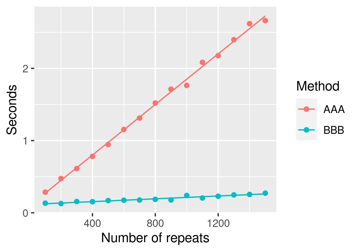
method,repeats,seconds
AAA,100,0.286
AAA,200,0.474
AAA,300,0.612
AAA,400,0.781
AAA,500,0.945
AAA,600,1.154
AAA,700,1.312
AAA,800,1.521
AAA,900,1.712
AAA,1000,1.764
AAA,1100,2.084
AAA,1200,2.177
AAA,1300,2.397
AAA,1400,2.619
AAA,1500,2.661
BBB,100,0.133
BBB,200,0.128
BBB,300,0.156
BBB,400,0.154
BBB,500,0.169
BBB,600,0.174
BBB,700,0.177
BBB,800,0.186
BBB,900,0.178
BBB,1000,0.240
BBB,1100,0.205
BBB,1200,0.229
BBB,1300,0.248
BBB,1400,0.254
BBB,1500,0.272
% Local Variables: % fill-column: 80 % End: