LaTeX notes
Table of Contents
- Quick links!
- Examples
- Latex notes
- Basic styling
- Help! Where is the manual?
- Lists
- Counting words with
texcount - Macros: probability and statistics
- Macros: referencing and linking
- Macros: genetic epidemiology
- Misc
- Math styling
- Writing new commands/macros
- Installation
- Help! I'm missing a package
- Basic usage
- Intermediate usage
- Proof reading and editing
- Bibliography
- Equations
- Typographic alignment
- Doublespacing
- Page numbers
- Timeline
- Figures
- Linking and referencing
- Tables
- Table of contents
- Table of special characters
- Authors and affiliations
- Bibtex notes
- TikZ notes
![]()
Quick links!
- Grab a copy of LoLTeX! My latex project set-up script.
- Grab a copy of my awesome beamer preamble.
- The LaTeX Wikibook.
- Table of fonts for mathematical symbols.
- Nick Higham's blog is a great source of LaTeX tips.
Examples
Standalone equation
\documentclass[preview,varwidth=true]{standalone}

\usepackage{amsmath}
\usepackage{amssymb}

\begin{document}

\begin{equation}
  h^2 = a^2 + b^2
\end{equation}

\end{document}
Standalone equation (again)
Here is a more involved example. This might be useful to include as an image in some slides.
\documentclass[preview,border=0.7cm,varwidth=11.8cm,convert={density=300,size=1080x800,outext=.png}]{standalone}

%% r0-in-words.tex
%% ===============
%%
%% This produces a simple image spelling out the effective
%% reproduction number of a birth-death-sampling model.
%%
%% Usage
%% -----
%%
%% pdflatex -shell-escape r0-in-words
%%

\usepackage{amsmath}
\usepackage{amssymb}
\usepackage{xcolor}

\begin{document}

{\fontfamily{phv}\fontsize{12}{10}\selectfont
  The \emph{effective reproduction number}, \(R\), is the expected number
  of secondary cases per infectious individual.

  \vspace{0.7cm}
  \noindent
  For the birth-death-sampling model
\begin{align*}
  R \quad=&\quad  \frac{\text{birth rate}}{\text{net removal rate}} \hspace{3.0cm} \\
  =& \quad\frac{\lambda}{\mu + \psi + \omega}
\end{align*}
}

\end{document}
To compile it, you need to allow -shell-escape to get PNG output.
pdflatex -shell-escape r0-in-words
Standalone references

\documentclass[
  preview,
  border=0.1cm,
  convert={density=300,outext=.png}
]{standalone}

%% bibliography-slide.tex
%% ======================
%%
%% Usage
%% -----
%%
%% To create a slide with the bibliography, run the following command:
%%
%% pdflatex bibliography-slide
%% pdflatex bibliography-slide
%% biber bibliography-slide
%% pdflatex -shell-escape bibliography-slide
%%
%% This will create a file called `bibliography-slide.png` which can
%% be included in a presentation. It reads the references from
%% references.bib

\usepackage{amsmath}
\usepackage{amssymb}
\usepackage{xcolor}

%% Since slides often use helvetica, these lines ensure the references
%% are printed in helvetica.
\usepackage[scaled]{helvet}
\renewcommand{\sfdefault}{phv}
\renewcommand{\familydefault}{\sfdefault}

\definecolor{camdarkblue}{HTML}{133844}

\usepackage[
  backend=biber,
  style=authoryear,
  dashed=false,
  maxcitenames=2,
  maxbibnames=2]{biblatex}
\addbibresource{bib-refs.bib}

%% The two numbers here are the fontsize (character size) and baseline
%% skip (spacing between lines). This is handled separately from the
%% main text font so needs to be defined here. A rule of thumb is that
%% the baseline skip should be 1.2 times the font size.
\renewcommand*{\bibfont}{\normalfont\fontsize{16pt}{19pt}\selectfont}

\begin{document}
%% The value given for the width of the minipage will be the width of
%% the resulting text.
\begin{minipage}{18cm}

{\color{camdarkblue}
\nocite{*}
\printbibliography[heading=none]
}

\end{minipage}
\end{document}
The following should be saved into references.bib
@article{stadler2009incomplete,
  title =        {{O}n incomplete sampling under birth-death models and
                  connections to the sampling-based coalescent},
  journal =      "Journal of Theoretical Biology",
  volume =       261,
  number =       1,
  pages =        "58--66",
  year =         2009,
  doi =          "10.1016/j.jtbi.2009.07.018",
  author =       "Tanja Stadler"
}

@article{stadler2010sampling,
  title =        {{S}ampling-through-time in birth-death trees},
  author =       "Tanja Stadler",
  journal =      "Journal of Theoretical Biology",
  volume =       267,
  number =       3,
  pages =        "396--404",
  year =         2010,
  doi =          "10.1016/j.jtbi.2010.09.010"
}

@article{stadler2011estimating,
  author =       {Stadler, Tanja and Kouyos, Roger and Bonhoeffer, Sebastian and
                  Joos, Beda and G\"{u}nthard, Huldrych F. and Rieder, Philip and
                  von Wyl, Viktor and Yerly, Sabine and B\"{o}ni, J\"{u}rg and
                  B\"{u}rgisser, Philippe and Klimkait, Thomas and Drummond, Alexei
                  J. and Xie, Dong and the Swiss HIV Cohort Study},
  title =        {{Estimating the Basic Reproductive Number from Viral Sequence
                  Data}},
  journal =      {Molecular Biology and Evolution},
  volume =       29,
  number =       1,
  pages =        {347-357},
  year =         2011,
  month =        09,
  issn =         {0737-4038},
  doi =          {10.1093/molbev/msr217}
}
Then to compile this use the following:
pdflatex bibliography-slide
pdflatex bibliography-slide
biber bibliography-slide
pdflatex -shell-escape bibliography-slide
Basic document I
See this example to extend this with a bibliography.
\documentclass[9pt,twocolumn]{scrartcl}
% \documentclass{article}

% ------------------------------------------------------------
% Packages
\usepackage{amsmath}
\usepackage{amssymb}
\usepackage[a4paper]{geometry}
\geometry{margin=0.75in}
\usepackage{hyperref}
% ------------------------------------------------------------

% ------------------------------------------------------------
% Macros
\newcommand{\name}[0]{}
% ------------------------------------------------------------

% ------------------------------------------------------------
% Title information
\title{Fleeb}
\date{}
\author{Squanchy}
% ------------------------------------------------------------

\begin{document}

\maketitle

Here is some text

\end{document}
You can use the article class for a more standard look, but I think the two
column scrartcl set up is very nice. I have also included some sections here
for stuff that is pretty standard and is useful to have as a reference. It won't
be terrible if you leave it in but do not need it.
The use of the geometry package means that you can use
\geometry{margin=0.75in} to utilise more of the page. I use this for two
columns so you may need to adjust it if you are using a single column.
Basic document II
LaTeX
Here is a basic LaTeX document that makes use of both images and references.
Note that it assumes the image is available in a directory called images.
\documentclass[fontsize=12pt,parskip=yes,onecolumn]{scrartcl}
% ------------------------------------------------------------
% Packages
\usepackage{amsmath}
\usepackage{amssymb}
\usepackage[a4paper]{geometry}
\geometry{margin=1.00cm}
\interfootnotelinepenalty=10000 % prevents footnote spreading across
% pages.
\usepackage{hyperref}
\usepackage[utf8]{inputenc}
\usepackage[english]{babel}
\usepackage{graphicx}
\usepackage[
natbib=true,
backend=bibtex,
maxcitenames=1,
minbibnames=3,
maxbibnames=40,
style=authoryear
]{biblatex}
\usepackage[
figurename=Figure,
font={sf,normalsize},
format=plain,
labelfont=bf,
]{caption}
\addbibresource{references.bib}
% ------------------------------------------------------------
% ------------------------------------------------------------
% Title information
\title{An example document}
\date{}
\author{Alexander E. Zarebski}
% ------------------------------------------------------------
\begin{document}
\maketitle
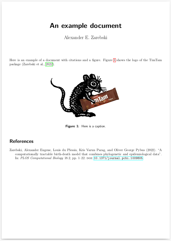
Here is an example of a document with citations and a figure.
Figure~\ref{fig:timtam} shows the logo of the TimTam package
\citep{zarebski2022computationally}. Doesn't it look nice?!
\begin{figure}[ht]
\centering
\includegraphics[width=0.5\linewidth]{images/timtam-beast2.png}
\caption{\label{fig:timtam} Here is a caption.}
\end{figure}
\printbibliography{}
\end{document}
Compilation
This can be compiled with the following script which also generates a date stamped PDF of the compiled document
#!/usr/bin/env bash
# -*- mode:sh; -*-

function compileAndClean {
    base_filename=$1
    # Compile LaTeX document
    pdflatex $base_filename
    bibtex $base_filename
    pdflatex $base_filename
    pdflatex $base_filename

    # List of extensions of temporary files to remove
    aux_extensions=(aux log out bbl blg run.xml)

    # Remove temporary files
    for ext in "aux_extensions[@]"; do
        tmp_file="$base_filename.$ext"
        if [ -f "$tmp_file" ]; then
            rm $tmp_file
        fi
    done

    # Make a backup copy of the pdf with today's date
    cp "$base_filename.pdf" "$base_filename-$(date '+%Y-%m-%d').pdf"
}

compileAndClean document
References
For completeness here is the Bibtex file called references.bib.
@article{zarebski2022computationally,
  doi =          {10.1371/journal.pcbi.1009805},
  author =       {Zarebski, {Alexander Eugene} AND {du Plessis}, Louis AND
                  Parag, {Kris Varun} AND Pybus, {Oliver George}},
  journal =      {PLOS Computational Biology},
  publisher =    {Public Library of Science},
  title =        {{A} computationally tractable birth-death model that combines
                  phylogenetic and epidemiological data},
  year =         2022,
  volume =       18,
  pages =        {1--22},
  number =       2
}
Bonus features
- Adding a macro to help with annotations is useful. I have an example here.
Letter I
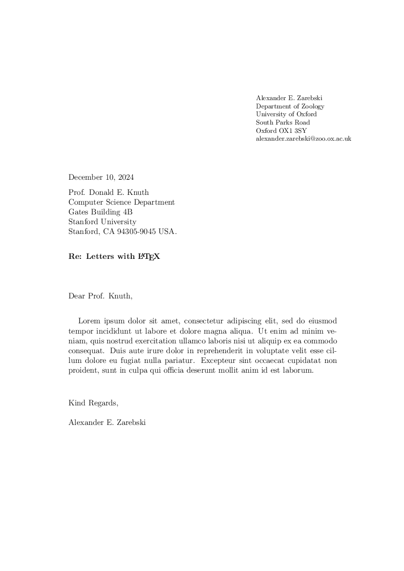
\documentclass[12pt,a4paper]{letter}

% -------------------------------------------------------------------------------
%       PAPER MARGINS
%-------------------------------------------------------------------------------

\textwidth 5.50in
\textheight 9.25in
\oddsidemargin 0.40in
\evensidemargin 0.00in
\topmargin -0.50in
\longindentation 0.50\textwidth
\parindent 0.2in

%-------------------------------------------------------------------------------
%       SENDER INFORMATION
%-------------------------------------------------------------------------------

\def\Who{Alexander E. Zarebski}
\def\Where{Department of Zoology\\University of Oxford}
\def\Address{South Parks Road}
\def\CityZip{Oxford OX1 3SY}
\def\Email{alexander.zarebski@zoo.ox.ac.uk}
% \def\URL{http://www.rmit.edu.au/}

%-------------------------------------------------------------------------------
%       HEADER AND FROM ADDRESS STRUCTURE
%-------------------------------------------------------------------------------

\address{
\hspace{5in}
\vskip -1.1in~\\
~\\[-0.11in]
\hspace{\fill}\parbox[t]{2.85in}{
\footnotesize
\Who \\
\Where\\
\Address\\
\CityZip\\
\Email\\
% \URL
}
\hspace{-1.3in} % Horizontal position of this block
\vspace{-1in}
}

%-------------------------------------------------------------------------------
%       TO ADDRESS STRUCTURE
%-------------------------------------------------------------------------------

\def\opening#1{\thispagestyle{empty}
{\centering\fromaddress \vspace{1.5in} \\
\today \hspace*{\fill}\par}
{\raggedright \toname \\ \toaddress \par}
\vspace{0.5in} % White space after the to address
\noindent #1
}

%-------------------------------------------------------------------------------
%       SIGNATURE
%-------------------------------------------------------------------------------

\signature{\Who}

\long\def\closing#1{
\vspace{0.2in}
\noindent
% \hspace*{\longindentation} % Move the signature right
\parbox{\indentedwidth}{\raggedright
#1 % Print the signature text
\vskip 0.2in % Whitespace between the signature text and your name
\fromsig}}

% -------------------------------------------------------------------------------

\begin{document}

%-------------------------------------------------------------------------------
%       TO ADDRESS
%-------------------------------------------------------------------------------

\begin{letter}
  {
    Prof. Donald E. Knuth \\
    Computer Science Department \\
    Gates Building 4B \\
    Stanford University \\
    Stanford, CA 94305-9045 USA. \\
    \vspace{0.3in}
    \textbf{Re: Letters with \LaTeX}}

%-------------------------------------------------------------------------------
%       LETTER CONTENT
%-------------------------------------------------------------------------------

\opening{Dear Prof. Knuth,}\\

Lorem ipsum dolor sit amet, consectetur adipiscing elit, sed do eiusmod tempor
incididunt ut labore et dolore magna aliqua. Ut enim ad minim veniam, quis
nostrud exercitation ullamco laboris nisi ut aliquip ex ea commodo consequat.
Duis aute irure dolor in reprehenderit in voluptate velit esse cillum dolore eu
fugiat nulla pariatur. Excepteur sint occaecat cupidatat non proident, sunt in
culpa qui officia deserunt mollit anim id est laborum.

\vspace{0.2in}
\closing{Kind Regards,}
%-------------------------------------------------------------------------------
\end{letter}
\end{document}
Letter II

\documentclass{letter}
\usepackage{graphicx}
\usepackage{lipsum}

% -------------------------------------------------------------------------------
%       PAPER MARGINS
%-------------------------------------------------------------------------------

\topmargin -0.70in
\textwidth 6.00in
\textheight 9.25in
\oddsidemargin 0.20in
\evensidemargin -0.20in

% -------------------------------------------------------------------------------
%       LETTER
%-------------------------------------------------------------------------------

\begin{document}

\begin{letter}{
    Admissions Committee \\
    Master of Science in Data Science Programme \\
    School of Computer Science and Engineering \\
    Nanyang Technological University \\
    Singapore}

\begin{minipage}[t]{0.48\textwidth}
    Dr Alexander E. Zarebski \\
    Lecturer in Applied Mathematics \\
    School of Mathematics \& Statistics \\
    University of Melbourne \\
    Peter Hall Building \\
    Parkville, VIC, 3010 \\
    Email: azarebski@unimelb.edu.au
\end{minipage}
\hfill
\begin{minipage}[t]{0.48\textwidth}
  \raggedleft
    \raisebox{-0.9\height}{\includegraphics[width=0.4\linewidth]{../resources/UoM_Logo_Vert_Housed_RGB.png}} % Adjust width as needed
\end{minipage}

\vspace{1cm}

\opening{Dear Admissions Committee,}
\vspace{5mm}

\lipsum[1-2] % Replace this with your actual letter content

\vspace{5mm}
\closing{Sincerely,\\[5mm]Alexander}

\end{letter}
\end{document}
Slides

\documentclass{beamer}
\usetheme{Madrid}
\usecolortheme{seagull}
\setbeamertemplate{navigation symbols}{}
\setbeamertemplate{footline}{}
\usefonttheme[onlymath]{serif}

\title{How to be cool}
\author{Arthur Herbert Fonzarelli}
\institute{Department of Cool, University of Cool}
\date{1 January 1974}

\begin{document}

\frame[plain]{\titlepage}

\begin{frame}[c]
  \frametitle{Foobar}
  123
\end{frame}

\begin{frame}[c]
  \frametitle{Barfoo}
  abc
\end{frame}

\end{document}
Pseudocode
Note that pseudocode is not the same as syntax highlighting; this example considers pseudocode, not real code. Installing the package can be a bit tricky, see the note below.
\documentclass[preview,varwidth=true]{standalone}

\usepackage{algorithm}
\usepackage{algorithmic}

\begin{document}

\begin{algorithmic}
\REQUIRE $n \geq 0$
\ENSURE $y = x^n$
\STATE $y \leftarrow 1$
\STATE $X \leftarrow x$
\STATE $N \leftarrow n$
\WHILE{$N \neq 0$}
\IF{$N$ is even}
\STATE $X \leftarrow X \times X$
\STATE $N \leftarrow N / 2$
\ELSE[$N$ is odd]
\STATE $y \leftarrow y \times X$
\STATE $N \leftarrow N - 1$
\ENDIF
\ENDWHILE
\end{algorithmic}

\end{document}
Installing the algorithm package
- Download the algorithms package from CTAN.
- Unzip it and within the resulting directory compile the
.styfiles withlatex algorithms.ins. - Copy the
.styfiles to the same directory as your.texand you can compile it withpdflatex.
(The dreaded) Gantt chart

\documentclass{standalone}
\usepackage{pgfgantt}

\begin{document}

\begin{ganttchart}[
  hgrid,
  vgrid,
  title/.style={fill=blue!20},
  title label font=\bfseries\color{black},
  bar/.style={fill=orange!50},
  bar height=0.7,
  group right shift=0,
  group height=.3,
  y unit chart=0.8cm
  ]{1}{12}

  \gantttitle{Week}{12} \\
  \gantttitlelist{1,...,12}{1} \\

  \ganttgroup{Preparation}{1}{3} \\
  \ganttbar{Choose recipe}{1}{1} \\
  \ganttbar{Buy ingredients}{2}{2} \\
  \ganttlinkedbar{Mix ingredients}{3}{3} \ganttnewline

  \ganttgroup{Baking}{4}{9} \\
  \ganttbar{Preheat oven}{4}{4} \\
  \ganttlinkedbar{Bake the cake}{5}{9} \ganttnewline

  \ganttgroup{Decoration}{10}{12} \\
  \ganttbar{Cool the cake}{10}{10} \\
  \ganttlinkedbar{Decorate the cake}{11}{12}
\end{ganttchart}

\end{document}
Latex notes
Basic styling
\underline{}\textbf{}\emph{}\hl{}which requires thesoulandcolorpackage (otherwise it just underlines)
Help! Where is the manual?
There is an unofficial reference manual that seems to be the best source of detailed information.
Lists
Customizing itemized lists: spacing
%% preamble
\usepackage{enumitem}

\begin{itemize}[topsep=-6pt, parsep=5pt]
\item foobar
\item foobar again
\end{itemize}
Or, to change the amount of indentation (i.e. the left margin) there is the following:
\usepackage{enumitem}

\setlist[itemize]{leftmargin=1em}
\setlist[description]{leftmargin=1em}
Customizing itemized lists: triangles
\usepackage{amsmath}
\usepackage{enumitem}
\setlist[itemize]{label=$\rhd$}
Customizing itemized lists: global spacing
\usepackage{enumitem}

\setlist[itemize]{
  label=$\rhd$,
  topsep=0pt,
  partopsep=0pt,
  parsep=5pt,
  itemsep=0pt
}
Counting words with texcount
The perl script texcount takes a .tex file and counts the number
of words that will be in the resulting PDF. You can get a copy by
installing texlive-utils-extra. Example output is shown below:
$ texcount manuscript.tex
File: manuscript.tex
Encoding: utf8
Words in text: 5205
Words in headers: 39
Words outside text (captions, etc.): 640
Number of headers: 17
Number of floats/tables/figures: 8
Number of math inlines: 102
Number of math displayed: 1
Subcounts:
  text+headers+captions (#headers/#floats/#inlines/#displayed)
  0+9+4 (1/0/0/0) _top_
  183+1+0 (1/0/0/0) Section: Abstract
  841+1+0 (1/0/5/0) Section: Introduction
  437+1+102 (1/1/10/0) Section: Methods
  1013+8+82 (3/1/59/1) Subsection: Likelihood function
  0+1+0 (1/0/0/0) Section: Results
  625+2+271 (1/4/10/0) Subsection: Simulation study
  435+9+100 (3/1/7/0) Subsection: SARS-CoV-2 on the Diamond Princess cruise ship
  544+5+81 (3/1/6/0) Subsection: Poliomyelitis in Tajikistan
  1057+1+0 (1/0/5/0) Section: Discussion
  70+1+0 (1/0/0/0) Section: Acknowledgements
Macros: probability and statistics
The following macros are useful for writing about probability and statistics and conform to the notation used in Bayesian Data Analysis where possible.
Note, when indicating a distribution restricted to taking positive
values, the convention here is to add a superscript + to the name of
the distribution. For example \(\text{Poisson}^{+}(\cdot)\) or \(\text{N}^{+}(\cdot,\cdot)\)
%% ============================================================
%% Distribution macros following the notation from BDA.
\newcommand{\Uniform}[2]{\text{U}\left(#1,#2\right)}
\newcommand{\Multinomial}[3]{\text{Multin}\left(#1,#2,\ldots,#3\right)}
\newcommand{\Normal}[2]{\text{N}\left(#1,#2\right)}
\newcommand{\Lognormal}[2]{\text{lognormal}\left(#1,#2\right)}
\newcommand{\GammaDist}[2]{\text{Gamma}\left(#1,#2\right)}
\newcommand{\Exponential}[1]{\text{Expon}\left(#1\right)}
\newcommand{\Beta}[2]{\text{Beta}\left(#1,#2\right)}
\newcommand{\Poisson}[1]{\text{Poisson}\left(#1\right)}
\newcommand{\Binomial}[2]{\text{Bin}\left(#1,#2\right)}
\newcommand{\NegativeBinomial}[2]{\text{Neg-bin}\left(#1,#2\right)}
\newcommand{\Prob}[1]{\text{Pr}\left(#1\right)}
\newcommand{\E}[2][]{\text{E}_{#1}\!\left(#2\right)}
\newcommand{\Variance}[1]{\text{var}\left(#1\right)}
\newcommand{\KLdiv}[2]{\text{KL}\left( #1 \middle\| #2 \right)}
%% ============================================================
Macros: referencing and linking
The following are some useful macros for referencing different elements of a document.
%% ============================================================
%% Macros for referencing things...
\newcommand{\Eqref}[1]{Eq.\eqref{#1}}
\newcommand{\Secref}[1]{\S\ref{#1}}
\newcommand{\Figref}[1]{Fig.\ref{#1}}
\newcommand{\Tabref}[1]{Table~\ref{#1}}
%% ============================================================
Macros: genetic epidemiology
%% ============================================================
\newcommand{\reff}[0]{\mathcal{R}_{\text{eff}}}
\newcommand{\refft}[1]{\mathcal{R}_{\text{eff}}(#1)}
\newcommand{\numPrev}[1]{N_{\text{prev}}(#1)}
\newcommand{\numCum}[1]{N_{\text{cum}}(#1)}
\newcommand{\tree}[0]{\mathcal{T}}
%% ============================================================
Misc
- use
a \gg banda \ll bto get \(a \gg b\) and \(a \ll b\).
Math styling
\underbrace{}_{}{n\choose x}for binomial coefficients\implies\boldsymbolfor bold math symbols
Writing new commands/macros
Here are a couple of simple examples.
\newcommand{\R}{\mathbb{R}}
\newcommand{\bb}[1]{\mathbb{#1}}
Installation
Don't forget to install all the extra stuff
sudo apt-get install texlive-full
Help! I'm missing a package
The following will install packages from CTAN
tlmgr install <PACKGENAME>
Basic usage
See the basic document example with, there is also a letter template there too.
Getting correct table and figure labels in supplementary files
Add the following to the preamble
% Make sure that both the tables and the figures have labels
% prefixed by a 'S'.
\let\oldthefigure\thefigure
\renewcommand{\thefigure}{S\oldthefigure}
\let\oldthetable\thetable
\renewcommand{\thetable}{S\oldthetable}
Compiling with bibtex
A typical compile.sh script will look like the following for a latex file
main.tex
MAIN_FILE=main

pdflatex $MAIN_FILE
pdflatex $MAIN_FILE
bibtex $MAIN_FILE
pdflatex $MAIN_FILE
Including line numbers
Adding the following lines to the preamble will include line numbers.
\usepackage{lineno}
\linenumbers
Intermediate usage
Page layout
The geometry package makes it easy to set the margins of the pages. In the
following, on line 1 the margin is used to set all margins to 7mm, and on line
2 the left and right margins are set to 5mm while the top and bottom are set to
10mm.
\geometry{margin=7mm} % 1
\geometry{hmargin=5mm,vmargin=10mm} % 2
Paragraph configuration
To set paragraph spacing and indentation, use the following in your
preamble (if you are using the article class).
\setlength{\parindent}{0pt}
\setlength{\parskip}{1em}
Using colour via xcolor
The following snippet defines the solarized colour palette which is a sensible starting point.
\usepackage{xcolor}

\definecolor{base03}{HTML}{002b36}
\definecolor{base02}{HTML}{073642}
\definecolor{base01}{HTML}{586e75}
\definecolor{base00}{HTML}{657b83}
\definecolor{base0}{HTML}{839496}
\definecolor{base1}{HTML}{93a1a1}
\definecolor{base2}{HTML}{eee8d5}
\definecolor{base3}{HTML}{fdf6e3}
\definecolor{yellow}{HTML}{b58900}
\definecolor{orange}{HTML}{cb4b16}
\definecolor{red}{HTML}{dc322f}
\definecolor{magenta}{HTML}{d33682}
\definecolor{violet}{HTML}{6c71c4}
\definecolor{blue}{HTML}{268bd2}
\definecolor{cyan}{HTML}{2aa198}
\definecolor{green}{HTML}{859900}
Including source code with syntax highlighting
This makes use of the colours defined above. This will provide reasonable highlighting for R code.
\usepackage{listings}

\lstset{
  language=R,
  linewidth=0.95\textwidth,
  xleftmargin=0.05\textwidth,
  basicstyle=\small\ttfamily\color{base02},
  backgroundcolor=\color{base3},
  showspaces=false,
  showstringspaces=false,
  showtabs=false,
  frame=single,
  frameround=tttt,
  float=p,
  rulecolor=\color{base03},
  tabsize=2,
  captionpos=b,
  breaklines=true,
  breakatwhitespace=false,
  keywordstyle=\color{base02},
  commentstyle=\color{base02},
  stringstyle=\color{cyan}
}
Making verbatim environments render nicely
Do yourself a favour and use the fancyvrb package. Here is a nice example
\begin{Verbatim}[frame=single,framerule=0.5mm,framesep=2mm,label=Git Usage,xleftmargin=5cm,xrightmargin=5cm]
year,percentage
2015,69.3
2017,69.2
2018,87.2
2020,82.8
2021,93.43
\end{Verbatim}
Compiling upon edits to files
You can recompile a PDF whenever a TeX file is updated using inotifywait as
described in my linux notes.
Proof reading and editing
Making notes on documents with a macro
The following is a useful way to make notes on a document. (You may also find this useful.)
\usepackage{todonotes}          % enable the use of \todo[]{}.
\newcommand{\mytodo}[1]{\todo[color=yellow, bordercolor=yellow, size=\tiny]{ #1 }}

\mytodo{Here is a note!}
Older versions of the package have poor support for colouring and shadows but the following example might be useful.
\usepackage[shadow]{todonotes}

% The colour support in todonotes is broken on the version of latex that is
% supported by Ubuntu 16.2 so you have to use this weird RGB + textcolor work
% around.

\definecolor{purple1}{rgb}{0.949, 0.941, 0.969}
% \definecolor{purple1}{HTML}{F2F0F7}
\definecolor{purple5}{rgb}{0.329, 0.153, 0.561}
% \definecolor{purple5}{HTML}{54278f}

\newcommand{\mytodo}[1]{\todo[
  color=purple1,
  bordercolor=purple5,
  size=\small,
  inline
  ]{\textcolor{purple5}{\sffamily FOOBAR: #1 }}}
Requesting a citations
Often you want to mark up a statement that requires a citation; here is a macro to help with that.
\newcommand{\aezcite}[0]{{\color{red}{\textbf{(CITE)}}}}
Viewing edits
Suppose you have an initial draft draft.tex and someone saves some revisions
to revisions.tex, you can get a marked up version of the differences with the
following
latexdiff draft.tex revisions.tex > diff.tex
pdflatex diff.tex
Warning! If you are using latexdiff it can get a bit cranky if you
change the layout of a table, for example by adding an extra column.
If you find yourself with this sort of problem, it is easiest to just
add an empty column in the same location in your original .tex file.
Strikeout and highlight macros
The mysout function is useful for indicating text for removal, and
the myhl one for indicating text that needs revision. It uses the
colour definitions from this snippet.
\usepackage{ulem}
\newcommand{\mysout}[1]{{\color{purple5}\sout{#1}}}
\newcommand{\myhl}[1]{{\colorbox{purple1}{#1}}}
Bibliography
Bibtex notes are here.
Equations
Putting a nice box around some equations
We can use the fancybox and empheq packages to create a nice box
around some equations.
\usepackage{empheq}
\usepackage{fancybox}
Note that we are setting the spacing around the box and the equations to be 10mm.
\setlength{\fboxsep}{10mm}
\begin{empheq}[box=\ovalbox]{align*}
\frac{ds}{dt} &= -\beta si\\
\frac{di}{dt} &= \beta si - \gamma i\\
\frac{dr}{dt} &= \gamma i
\end{empheq}
Aligning multiple equations without an equation label
Remember to include \bverb|amsmath| in your preamble. The following example demonstrates how to align multiple equations.
\begin{align*}
f(0) = f(1) &= 1 \\
f(n) &= f(n-1) + f(n-2)
\end{align*}
Aligning multiple equations with an equation label
\begin{equation}\label{eq:foo}
  \begin{aligned}
    f(0) = f(1) &= 1 \\
    f(n) &= f(n-1) + f(n-2)
  \end{aligned}
\end{equation}
N.b. using align* in place of aligned here is considered bad
practise, but both will achieve the desired result.
Piece-wise defined functions
The following example is taken from a tex.stackexchange answer
\usepackage{amsmath}

\[ f(x) = \begin{cases}
      0 & x\leq 0 \\
      \frac{100-x}{100} & 0\leq x\leq 100 \\
      0 & 100\leq x
   \end{cases}
\]
Referencing equations
If you need to reference equations, the following macro might be
useful. N.b. \eqref is the same as \ref but it puts parenthesis
around the equation number to emphasize that it is an equation.
\usepackage{amsmath}

\newcommand{\Eqref}[1]{Equation~\eqref{#1}}

%% Additional ones for sections and figures...
\newcommand{\Secref}[1]{\S~\ref{#1}}
\newcommand{\Figref}[1]{Fig~\ref{#1}}
Typographic alignment
- ragged right (flush left)
- text aligns to left margin with constant word spacing. There is a preference for this for accessibility.
- justified
- test aligns to both left and right margin with variable word spacing
- ragged left (flush right)
- text aligns to right margin with constant word spacing
- centered
- constant spacing, symmetric about middle of the column
Ragged right
% Preamble
\usepackage{ragged2e}

% ...

\begin{document}
\RaggedRight
Doublespacing
To use doublespacing for lines add the following line to your preamble.
\usepackage[doublespacing]{setspace}

% or

\usepackage{setspace}
\doublespacing
Page numbers
To remove page numbers include the nopageno package
\usepackage{nopageno}
Timeline
Taken from this stackoverflow answer by Fran.
\documentclass{article}
\usepackage{xcolor}
\newcommand\ytl[2]{
\parbox[b]{8em}{\hfill{\color{cyan}\bfseries\sffamily #1}~$\cdots\cdots$~}\makebox[0pt][c]{$\bullet$}\vrule\quad \parbox[c]{4.5cm}{\vspace{7pt}\color{red!40!black!80}\raggedright\sffamily #2.\\[7pt]}\\[-3pt]}
\begin{document}
\begin{table}
\caption{Timeline of something.}
\centering
\begin{minipage}[t]{.7\linewidth}
\color{gray}
\rule{\linewidth}{1pt}
\ytl{1947}{AT and T Bell Labs develop the idea of cellular phones}
\ytl{1968}{Xerox Palo Alto Research Centre envisage the `Dynabook'}
\ytl{1971}{Busicom 'Handy-LE' Calculator}
\ytl{1973}{First mobile handset invented by Martin Cooper}
\ytl{1978}{Parker Bros. Merlin Computer Toy}
\ytl{1981}{Osborne 1 Portable Computer}
\ytl{1982}{Grid Compass 1100 Clamshell Laptop}
\ytl{1983}{TRS-80 Model 100 Portable PC}
\ytl{1984}{Psion Organiser Handheld Computer}
\ytl{1991}{Psion Series 3 Minicomputer}
\bigskip
\rule{\linewidth}{1pt}%
\end{minipage}%
\end{table}
\end{document}
Figures
Replacing graphics with placeholders for drafts
You can replace figures with an empty box (of the correct size)
containing the name of the filepath during the drafting process by
giving the draft argument to the graphicx package as shown in the
following example:
\usepackage[draft]{graphicx}
This is useful, because compiling a PDF without the figures can be many times faster than compiling with the figures (depending on how many figures and how large the files are).
Setting the graphics path
Suppose your figures live in a directory img. To include these
figures, add the following to the preamble
\usepackage{graphicx}
\graphicspath{ {./images/} }
then to include a figure in the document use the following
\begin{figure}
  \centering
  \includegraphics[width=.7\linewidth]{name-of-figure-file}
  \caption{Here is a caption}
  \label{fig:figure-label}
\end{figure}
Cropping graphicss
You can crop the imported graphic:
\includegraphics[trim=left bottom right top, clip]{file}
Making figure captions look nice
- See here for information about table labels.
The following usage of the caption package tweaks the formatting of
figure captions to distinguish them from the main text.
\usepackage[
figurename=Figure,
font={sf,small},
format=plain,
labelfont=bf,
]{caption}
fontspecifies to use a small sans-serif font.labelfontsays to show the figure label in bold and thefigurenamedeclares that we want this labelled as a "Figure".
Linking and referencing
Within-document references
To label a section use \label{sec:cool-name} and to refer to link to it later
use \ref{sec:cool-name}. The sec: prefix is not necessary, but it makes
things clearer.
For finer control there is also the functions hypertarget and hyperlink
provided by the hyperref package.
Linking to URL
The hyperref package provides functions to assist in generating hyperlinks.
\href{https://aezarebski.github.io}{Amazing}
\url{https://aezarebski.github.io}
Style of figure labels
By default figures and tables are labelled with arabic numerals, eg "Figure 1". If you want to prefix these numbers with the letter 'S' for figures in the supplement, then you can use the following:
\renewcommand{\thetable}{S\arabic{table}}
\renewcommand{\thefigure}{S\arabic{figure}}
If instead you want to label them with letters — which is what PLOS Comput. Biol. requests — then the following might help.
\renewcommand{\thefigure}{\Alph{figure}}
\renewcommand{\thetable}{\Alph{table}}
Tables
- See here for information about table labels.
\begin{table}
  \caption{\label{tab:demo}Go tabular data!}
  \centering
  \fbox{
    \begin{tabular}{lll}
Sepal Length & Sepal Width & Species\\
\hline
5.1 & 3.5 & setosa\\
4.9 & 3.0 & setosa\\
    \end{tabular}
  }
\end{table}
You can also use the fantastic Tables Generator webapp.
Wrapped text
\begin{tabular}{|p{1cm}|p{3cm}|}
  This text will be wrapped & Some more text \\
\end{tabular}
Table of contents
To add a table of contents, use \tableofcontents at the start of the
document.
To adjust the depth to which sections are numbered, add the following
to the preamble. The secnumdepth describes depth of numbering to
include (e.g., 1 gives \(n\), 2 gives \(n.m\), etc.)
\setcounter{secnumdepth}{2}
To adjust the depth of the sections displayed in the table of
contents, add the following to the preamble. The tocdepth describes
the depth of sections to display (e.g., 1 gives sections only, 2
gives sections and subsections, etc.)
\setcounter{tocdepth}{2}
Table of special characters
The Wikibook has a full table of special characters, here are some that I need on the regular:
| Latex | Description | Sample |
|---|---|---|
\'{o} |
Acute accent | ó |
\^{o} |
Circumflex | ô |
\"{o} |
Umlaut | ö |
\c{c} |
Cedilla | ç |
\r{a} |
Ring over letter | å |
\o{} |
o with strike | ø |
Authors and affiliations
This is a minimal example demonstrating how to include multiple authors with their own affiliations.
\documentclass{article}

\usepackage{authblk}            % provides author affiliations.

\title{Fleeb}
\date{}
\author[1]{Morty Smith\thanks{For correspondence email: yolo@hotmail.com}}
\author[2]{Rick Sanchez}
\affil[1]{Princeton University}
\affil[2]{School of Hard Knocks}

\begin{document}

\maketitle

Here is some text

\end{document}
Bibtex notes
![]()
GUI: Jabref
![]()
- A GUI for managing bibtex files.
- Download it from here.
- Set your Bibtex key pattern to
[auth:lower][year][veryshorttitle:lower]. - The
--prexpand--primpallow you to export and import your configuration (respectively) from an XML file.
TODO Summary of bib file
Extract used citations
The script will print out all of the citations that have been used in a tex file which can be useful when fiddling around with bibtex stuff.
library(argparse)

parser <- ArgumentParser()
parser$add_argument(
         "tex",
         default = "",
         help = "Input tex file."
       )

main <- function(args) {
  input_tex <- args$tex

  if (!file.exists(input_tex)) {
    stop("Could not find given file: ", input_tex)
  }

  tex_lines <- readLines(input_tex)

  non_comments <- grep(
    pattern = "^%",
    x = tex_lines,
    value = TRUE,
    invert = TRUE)

  cite_pattern <- "[[:alpha:]]+[[:digit:]]+[[:alpha:]]*"
  pattern <- sprintf("%s(,[ ]*%s)*", cite_pattern, cite_pattern)
  matches <- regmatches(non_comments, regexpr(pattern, non_comments))

  for (m in matches) {
    if (grepl(pattern = ",", x = m)) {
      for (mx in unlist(strsplit(x = m, ","))) {
        cat(mx, "\n")
      }
    } else {
      cat(m, "\n")
    }
  }
}

if (!interactive()) {
  args <- parser$parse_args()
  main(args)
}
BBL files and PLOS madness
PLOS journals require that you don't use a .bib file, instead they want you to
compile a .bbl file and copy the contents of that into your .tex file at the
end. An easy way to do this is outlined in the following stackexchange post:
https://tex.stackexchange.com/a/329201
Basically, this involves compiling a document from the following file where your
references are in references.bib and then using the generated .bbl file.
\documentclass[10pt,a4paper]{article}

\usepackage{hyperref} % for better urls


\begin{document}

This is text with \cite{foo1984bar}.

\nocite{*} % to test all bib entrys
\bibliographystyle{plos2015}
\bibliography{references} % file mwe.bib

\end{document}
If this is saved as demo.tex then you would make demo.bbl with the following
commands
pdflatex demo
bibtex demo
pdflatex demo
pdflatex demo
Citation command
There are two main commands for citation: citet and citep since cite is
pretty much an alias of cite. The citep command is used for parenthetical
citations and the citet is for when the citation is included as part of the
sentence in which it appears.
Format examples
There are a bunch of useful examples available via yasnippet, I couldn't work out which package they come from, but they are there and very useful.
Newspaper article
For an online article, the following entry type can be used
@article{lastname2021something,
  author  = {Smith, Alex},
  title   = {Something important happened},
  date    = {2021-03-02},
  journal = {BBC News},
  url     = {https://www.bbc.co.uk/news/blahblahblah},
  urldate = {2021-03-02}
}
The misc example may be useful if the publication method is less formal.
Technical report
@techreport{techreport,
  author =       {{Grabm{\"u}ller, Martin}},
  title        = {{M}onad {T}ransformers {S}tep by {S}tep},
  year         = 2006,
  note         = {Available in draft}
}
The unpublished format is pretty much the same.
Miscellaneous
@misc{graham2021how,
  author =       {Graham, Paul},
  title =        {{H}ow to {W}ork {H}ard},
  month =        {June},
  year =         2021,
  howpublished = {Available at \url{http://paulgraham.com/hwh.html}
                  (2021/06/30)}
}
This might be useful for blog posts and essays, although for news items see this example.
Example: Basic nice usage
\documentclass{article}
\usepackage[utf8]{inputenc}
\usepackage[english]{babel}

\usepackage[
natbib=true,
backend=bibtex,
maxcitenames=2,
style=authoryear
]{biblatex}

\addbibresource{references.bib}

\begin{document}

foobar

\printbibliography{}

\end{document}
The alphabetic style is the initials of the first author and the year.
Example: references when you are short on space
This is the same as the nice example above, but uses numeric-comp
and some other tweaks to reduce the amount of space used by the
references.
\usepackage[
natbib=true,
backend=bibtex,
maxcitenames=1,
minbibnames=1,
maxbibnames=1,
style=numeric-comp
]{biblatex}
\renewcommand{\bibfont}{\small}        % small font (approx 10pt)
\defbibheading{bibliography}[\relax]{} % remove title
\setlength{\bibitemsep}{0mm}    % spacing
Character encoding trouble
If you are getting errors about there being non-ASCII characters in your
bibtex file, the following command can help you to find them.
LANG=C grep --color=always '[^ -~]\+' <path/to/bibliography.bib>
TikZ notes
Overleaf has a good TikZ introduction.
Environment
\documentclass[preview]{standalone}
\usepackage[utf8]{inputenc}

\usepackage{tikz}
\usetikzlibrary{positioning}

\begin{document}

\begin{figure}
  \begin{tikzpicture}

    % Put the marvelous tikz diagram code here!!!

  \end{tikzpicture}
\end{figure}

\end{document}
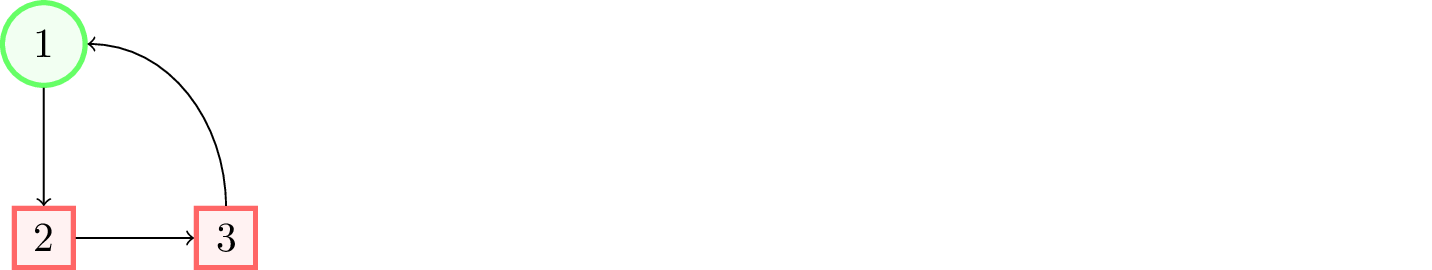
Example: basic diagram
\begin{tikzpicture}[
  roundnode/.style={circle, draw=green!60, fill=green!5, very thick, minimum size=7mm},
  squarednode/.style={rectangle, draw=red!60, fill=red!5, very thick, minimum size=5mm},
  ]

  % Nodes
  \node[squarednode]      (maintopic)                              {2};
  \node[roundnode]        (uppercircle)       [above=of maintopic] {1};
  \node[squarednode]      (rightsquare)       [right=of maintopic] {3};

  % Lines
  \draw[->] (uppercircle.south) -- (maintopic.north);
  \draw[->] (maintopic.east) -- (rightsquare.west);
  \draw[->] (rightsquare.north) .. controls +(up:7mm) and +(right:7mm) .. (uppercircle.east);

\end{tikzpicture}
There are definitions of how to draw roundnode and squarednode, followed by
the declarations of these nodes in the diagram and the lines to draw between
them. This compiles with pdflatex to give the following