AANN 02/05/2024

In this example we will use the Optuna hyperparameter optimization framework (Akiba et al (2019)) to optimise the training and structure of a simple model for MNIST classification. This is largely based on an example from Optuna's GitHub repository.

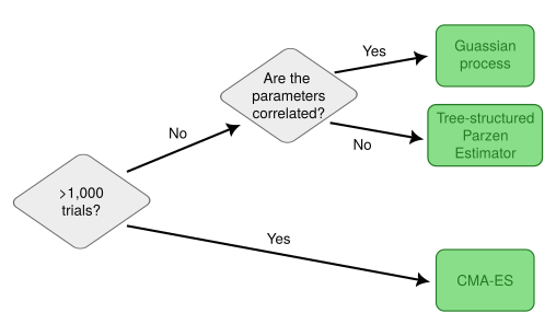
In hyperparameter optimization, the objective function is the validation score of a model as a function of the hyperparameters used to train it. Akiba et al suggest, at a technical level, this requires good algorithms for two things: sampling and pruning. Sampling refers to choosing the next set of hyperparameters to trial based on the results of previous trials. For example, a Gaussian process can be used to approximate the objective function. A decision tree for how to select the sampling algorithm is given in Figure 1. Pruning refers to the process of terminating a trial early if it becomes clear the current hyperparameters are bad. Pruning is important because it means those computational resources can be allocated to more promising configurations.

The full script with all the code is here.

import optuna

def objective(trial):
    x = trial.suggest_float('x', -10, 10)
    return (x - 2) ** 2

study = optuna.create_study()
study.optimize(objective, n_trials=100)

study.best_params  # E.g. {'x': 2.002108042}

INPUT_SIZE= 28 * 28
CLASSES = 10

def define_model(trial):
    n_layers = trial.suggest_int("n_layers", 1, 3)
    layers = []

    in_features = INPUT_SIZE
    for i in range(n_layers):
        out_features = trial.suggest_int("n_units_l{}".format(i), 4, 128)
        layers.append(nn.Linear(in_features, out_features))
        layers.append(nn.ReLU())
        p = trial.suggest_float("dropout_l{}".format(i), 0.2, 0.5)
        layers.append(nn.Dropout(p))
        in_features = out_features

    layers.append(nn.Linear(in_features, CLASSES))
    layers.append(nn.LogSoftmax(dim=1))
    return nn.Sequential(*layers)

trial.report(validation_loss, epoch)
if trial.should_prune():
    raise optuna.exceptions.TrialPruned()

def objective(trial):
    model = define_model(trial).to(DEVICE)

    optimizer_name = trial.suggest_categorical("optimizer", ["Adam", "SGD"])
    lr = trial.suggest_float("lr", 1e-5, 1e-1, log=True)
    optimizer = getattr(optim, optimizer_name)(model.parameters(), lr=lr)

    train_loader, valid_loader = get_mnist()

    for epoch in range(EPOCHS):
        model.train()
        for batch_idx, (data, target) in enumerate(train_loader):
            data, target = data.view(data.size(0), -1).to(DEVICE), target.to(DEVICE)
            optimizer.zero_grad()
            output = model(data)
            loss = LOSS_FN(output, target)
            loss.backward()
            optimizer.step()

        model.eval()
        validation_loss = 0
        with torch.no_grad():
            for batch_idx, (data, target) in enumerate(valid_loader):
                data, target = data.view(data.size(0), -1).to(DEVICE), target.to(DEVICE)
                output = model(data)
                loss = LOSS_FN(output, target)
                validation_loss += loss.item()

        trial.report(validation_loss, epoch)
        if trial.should_prune():
            raise optuna.exceptions.TrialPruned()

    return validation_loss

study = optuna.create_study()
study.optimize(objective, n_trials=100, timeout=600)

optuna.visualization.plot_optimization_history(study)

The results of this optimization are summarised by the following print out. Perhaps surprisingly, this favoured a single layer model with 79 units.

Study statistics:
  Number of finished trials:  28
  Number of pruned trials:  9
  Number of complete trials:  19
Best trial:
  Value:  7.240957830101252
  Params:
    n_layers: 1
    n_units_l0: 79
    dropout_l0: 0.2814220675694274
    optimizer: Adam
    lr: 0.004062149899383117

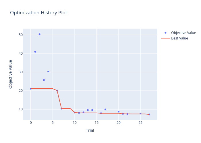
Figure 2 shows the values of the objective function across the trials of the study, highlighting how the optimal solution has progressed. The red line indicates the best performance seen up until that point in the study.

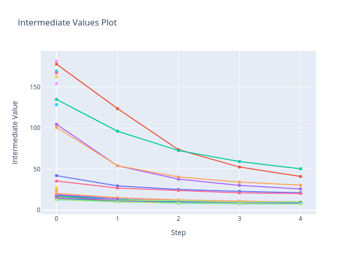
Figure 3 zooms in on each of the trials, showing how the optimisation process unfolded. There are some points in this figure that do not have subsequent evaluations. These isolated points are where the pruning algorithm has terminated the trial early to use the computational resources elsewhere. The values for this plot comes from the report values, (see the end of the objective function above). Note that the first evaluation comes after a complete epoch of training which is why some start off so much better than the others.

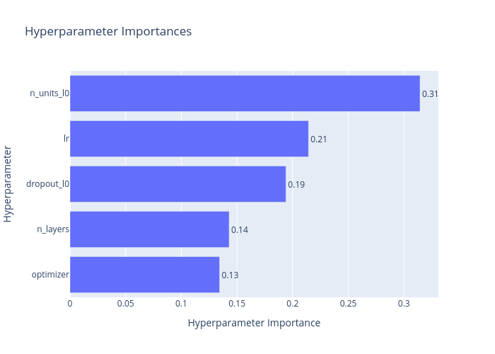
Finally, and perhaps most importantly for the subsequent optimisation, Figure 4 ranks the variables being optimised in terms of importance.

I found Optuna very easy to use with a well-thought-out API which covered everything I need and more (there is also a fancy web-dashboard, but I haven't tried that.) This example is probably too small to demonstrate the use of the package properly, but should give a good idea of how it works.