AANN 25/01/2024

Simultaneous quantile regression

In this example we will use the simultaneous quantile regression (SQR) as proposed by Tagasovska and Lopez-Paz (2019) to compute the quantiles of a prediction. SQR provides a way to get a prediction with a quantification of the uncertainty in that prediction. If you want to get technical, this is an instance of aleatoric uncertainty (i.e. the uncertainty intrinsic to a known stochastic process), as opposed to epistemic uncertainty (i.e. the uncertainty that derives from possible model misspecification.) Since I am mainly interested in the aleatoric uncertainty, I will ignore the orthonormal certificates that Tagasovska and Lopez-Paz proposed as a way to manage the epistemic uncertainty.

We will use SQR to estimate the quantiles of a distribution. Since the use of SQR is primarily about the loss function used in the optimisation, (not the network architecture itself), we will just use a simple feed-forward network to generate the estimates. We will also use simulated data so we have a known "truth" to compare to.

Data generating process

The input to our neural network is a datum, \(x_i=(x_i^1,\ldots,x_i^m)\), where

\[ x_i^j\sim\text{Normal}(\mu_i,1) \]

for \(j=1,\ldots,m\). Our goal is to use a set of observations, \(x_i\) to predict \(y_i=\mu_i\) where we assume a prior distribution \(\mu_i\sim\text{Normal}(0,10)\). This model is simple enough that we can calculate the quantiles analytically.

Loading packages

PyTorch has some nice random number generation functionality and this saves us needing to put the values into tensors later. We set the seed to keep things reproducible.

import time
import sys
import os
from pathlib import Path

import torch
import torch.nn as nn
import torch.optim as optim
from torch.distributions import normal, uniform
import pandas as pd
import plotnine as p9
from plotnine import *

current_directory = Path(os.getcwd())
sys.path.append(str(current_directory.parent))
import niceneuron.plot as nn_plot
torch.manual_seed(0)

Define the input and output filenames

There is a replicate_size (in addition to a number of replicates) because we are using a permutation invariant network similar to the previous post, and each data point consists of a set of observations.

loss_png = "loss.png"
loss_csv = "loss.csv"
coverage_png = "coverage.png"

replicate_size = 10

train_num_replicates = 10000
train_num_steps = 10000
train_record_every = 500

test_num_replicates = 100

Define the network architecture

The network we will use is based on the one from the previous post.
We call the network LocationNB because it estimates the location parameter of a sample and is reminiscent of the neural Bayes structure.
To ensure it is permutation invariant we compute three summary statistics as a preprocessing step: the median and the first and second moments.
A value for tau is given as input so the network knows what quantile to compute.

class LocationNB(nn.Module):
    def __init__(self, m):
        super(LocationNB, self).__init__()
        self._m = m      # dataset size: {z_1,...,z_m}
        self._num_S = 3  # number of summary statistics
        self._q = 10     # latent dimension
        self._p = 1      # output dimension

        self._phi = nn.Sequential(
            nn.Linear(self._num_S + 1, self._q),
            nn.Sigmoid(),
            nn.Linear(self._q, self._p),
        )

    def signed_sqrt(self, x):
        return torch.sign(x) * torch.sqrt(torch.abs(x))

    def forward(self, x, tau):
        # assert x.dim() == 2 and x.shape[1] == self._m
        # assert tau.dim() == 1 and x.shape[0] == tau.shape[0]

        s0 = torch.median(x, dim=1).values
        s1 = torch.mean(x, dim=1)
        s2 = torch.mean(x**2, dim=1)
        tmp = torch.stack([s0, s1, s2], dim=1)
        tmp = self.signed_sqrt(tmp)
        tmp = torch.cat([tmp, tau.unsqueeze(1)], dim=1)
        return self._phi(tmp).squeeze(1)

Define the pinball loss function

We define the pinball loss as a PyTorch loss function so the network can learn to predict quantiles. To see why this function yields the quantile estimator you need to solve for the root of the derivative. Mathematically, the loss function \(\ell_{\tau}\) associated with a prediction of \(\hat{y}\) for a true value of \(y\) is

\[ \ell_{\tau}(\hat{y}, y) =\begin{cases} \tau (y - \hat{y}) & \text{if } y \geq \hat{y} \\ (1 - \tau) (\hat{y} - y) & \text{if } y < \hat{y} \end{cases} \]

IMPORTANT: This definition allows for the use of a different value of \(\tau\) for each element of the target tensor. This is the distinguishing factor of simultaneous quantile regression. Training the network to learn multiple quantiles simultaneously purportedly provides a partial resolution to the crossing quantile problem where the ordering of the quantiles is not respected.

class PinballLoss(nn.Module):
    def __init__(self):
        super(PinballLoss, self).__init__()

    def forward(self, predictions, targets, tau):
        err = targets - predictions
        loss = torch.where(err >= 0, tau * err, (tau - 1) * err)
        return torch.mean(loss)

Define data generating process

Because we are going to need separate training and testing datasets, it is helpful to have a function that makes it easy to simulate new data.

def rand_dataset(num_replicates: int, replicate_size: int):
    mu_i = normal.Normal(torch.tensor([0.0]), torch.tensor([10.0])).sample(
        sample_shape=torch.Size([num_replicates])
    )
    x_i = (
        normal.Normal(loc=mu_i, scale=torch.tensor([1.0]))
        .sample(sample_shape=torch.Size([replicate_size]))
        .transpose(0, 1)
        .squeeze(2)
    )
    y_i = mu_i.squeeze(1)
    return y_i, x_i

Prepare for training

Because it worked out of the box, I didn't see much need to go beyond a standard Adam optimizer.

loc_nb = LocationNB(replicate_size)

pb_loss = PinballLoss()

optimizer = optim.Adam(loc_nb.parameters(), lr=1e-3)

Run the training loop

At each step of the optimisation we simulate a new data set so we don't need to worry about shuffling or precomputing all the data beforehand. It would be nice to extend this to include a stopping criterion.

loc_nb.train()
loss_history = []
training_start_time = time.time()
for step in range(train_num_steps):
    # Sample training data
    train_y, train_x = rand_dataset(train_num_replicates, replicate_size)
    train_tau = (
        uniform.Uniform(torch.tensor([0.0]), torch.tensor([1.0]))
        .sample(sample_shape=train_y.shape)
        .squeeze(1)
    )
    # Forward pass
    preds = loc_nb(train_x, train_tau)
    loss = pb_loss(preds, train_y, train_tau)
    step_loss = loss.item()

    # Backward pass
    optimizer.zero_grad()
    loss.backward()
    optimizer.step()

    if step % train_record_every == 0:
        print(f"Step {step} loss: {step_loss}")
        loss_history.append((step, step_loss))
training_finish_time = time.time()
print(f"Training took: {training_finish_time - training_start_time}")

Visualise training results

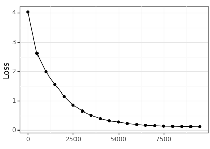
We can visualise the training error across the steps of the optimisation.

loss_df = pd.DataFrame(loss_history, columns=["step", "loss"])
loss_df.to_csv(loss_csv)
loss_p9 = nn_plot.plot_loss_curve(loss_df, x_var="step", x_lab="")
loss_p9.save(loss_png, height = 2.9, width = 4.1)

Test the network performance

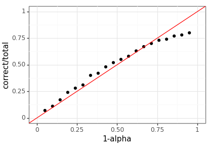
To test how well-calibrated the predicted quantiles are we generate a large dataset and then investigate how often the empirical quantiles match up with the desired ones. The performance is great, but by no means perfect.

test_y, test_x = rand_dataset(test_num_replicates, replicate_size)
test_alpha = torch.linspace(0.05, 0.95, steps=20)
test_results = []

for ix in range(test_alpha.shape[0]):
    tau_0 = (0.5 * test_alpha[ix]).repeat(test_num_replicates)
    tau_1 = 1 - tau_0
    test_est_lower = loc_nb(test_x, tau_0)
    test_est_upper = loc_nb(test_x, tau_1)
    test_correct = torch.sum(
        (test_est_lower <= test_y) & (test_y <= test_est_upper)
    ).item()
    test_results.append((test_alpha[ix].item(), test_correct, test_num_replicates))

Visualisation

test_df = pd.DataFrame(test_results, columns=["alpha", "correct", "total"])

(
    ggplot(test_df, aes(x="1-alpha", y="correct/total"))
    + geom_point()
    + geom_abline(intercept=0, slope=1, color="red")
    + scale_x_continuous(limits=(0, 1))
    + scale_y_continuous(limits=(0, 1))
    + theme_bw()
).save(coverage_png, height=2.9, width=4.1)

Discussion

Simultaneous quantile regression produces a generic quantile regression model. However, the method lacks finite-sample guarantees. Quantile regression can be combined with conformal prediction to yield conformalized quantile regression to overcome this limitation (as described by Romano et al (2019)).

Thanks

Thanks to Jackson Kwok for helpful comments on a draft of this.