latex-gallery-aez
![]()
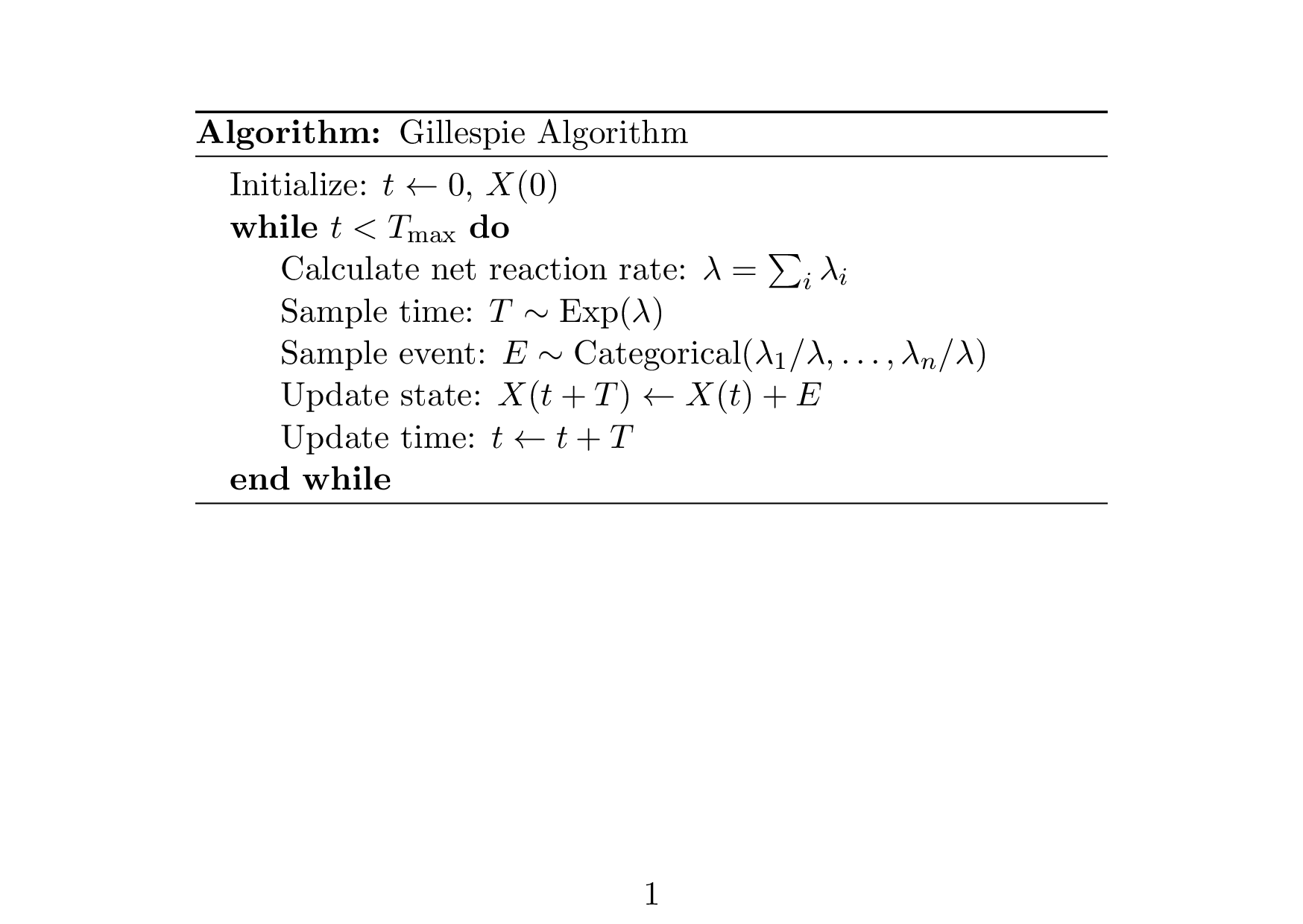
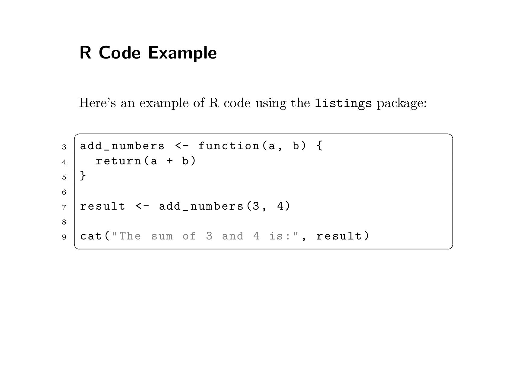


Figure 1
Keywords: Algorithm, Code
\documentclass{scrartcl}
\usepackage{algorithm}
\usepackage{algpseudocode}
\usepackage{caption}
\usepackage{amsmath}
\usepackage[landscape,a6paper]{geometry}

%% Remove number from algorithm title
\DeclareCaptionLabelFormat{nonumber}{#1:}
\captionsetup[algorithm]{labelformat=nonumber}

\begin{document}

\begin{algorithm}
\caption{Gillespie Algorithm}\label{alg:gillespie}
\begin{algorithmic}[0]          % argument 1 for numbered lines
  \State Initialize: $t \gets 0$, $X(0)$

  \While{$ t < T_{\max} $}
  \State Calculate net reaction rate: \(\lambda = \sum_{i} \lambda_{i}\)
  \State Sample time: \(T \sim \text{Exp}(\lambda)\)
  \State Sample event:
  \(E \sim \text{Categorical}(\lambda_{1} /\lambda, \ldots, \lambda_{n}/\lambda)\)
  \State Update state: \(X(t + T) \gets X(t) + E\)
  \State Update time: $t \gets t + T$
  \EndWhile

\end{algorithmic}
\end{algorithm}

\end{document}
Figure 2
Keywords: Source code, R
\documentclass{scrartcl}
\usepackage[landscape,a6paper]{geometry}
\pagestyle{empty}
\usepackage{xcolor}
\usepackage{listings}

\lstdefinestyle{RStyle}{
  language=R,
  basicstyle=\small\ttfamily,
  stringstyle=\color{gray},
  numbers=left,
  numberstyle=\tiny,
  firstnumber=3,
  showstringspaces=false,
  frame=single,
  frameround=tttt
}

\begin{document}

\section*{R Code Example}

\vspace{5mm}

Here's an example of R code using the \texttt{listings} package:

\vspace{5mm}

\begin{lstlisting}[style=RStyle]
add_numbers <- function(a, b) {
  return(a + b)
}

result <- add_numbers(3, 4)

cat("The sum of 3 and 4 is:", result)
\end{lstlisting}

\end{document}
convert -density 300 -colorspace RGB -background white -alpha remove -alpha off input.pdf output.png
Figure 3
Keywords: References, slides
\documentclass[
  preview,border=0.7cm,varwidth=12.8cm,
  convert={density=300,size=1080x800,outext=.png}]{standalone}

%% bibliography-slide.tex
%% ======================
%%
%% Usage
%% -----
%%
%% To create a slide with the bibliography, run the following command:
%%
%% pdflatex bibliography-slide
%% pdflatex bibliography-slide
%% biber bibliography-slide
%% pdflatex -shell-escape bibliography-slide
%%
%% This will create a file called `bibliography-slide.png` which can
%% be included in a presentation. It reads the references from
%% references.bib

\usepackage{amsmath}
\usepackage{amssymb}
\usepackage{xcolor}

%% Since slides often use helvetica, these lines ensure the references
%% are printed in helvetica.
\usepackage[scaled]{helvet}
\renewcommand{\sfdefault}{phv}
\renewcommand{\familydefault}{\sfdefault}

\usepackage[
  backend=biber,
  style=authoryear,
  dashed=false,
  maxcitenames=2,
  maxbibnames=2]{biblatex}
\addbibresource{references.bib}

\begin{document}

\printbibliography[heading=none]
\nocite{*}

\end{document}
@article{stadler2009incomplete,
  title =        {{O}n incomplete sampling under birth-death models and
                  connections to the sampling-based coalescent},
  journal =      "Journal of Theoretical Biology",
  volume =       261,
  number =       1,
  pages =        "58--66",
  year =         2009,
  doi =          "10.1016/j.jtbi.2009.07.018",
  author =       "Tanja Stadler"
}

@article{stadler2010sampling,
  title =        {{S}ampling-through-time in birth-death trees},
  author =       "Tanja Stadler",
  journal =      "Journal of Theoretical Biology",
  volume =       267,
  number =       3,
  pages =        "396--404",
  year =         2010,
  doi =          "10.1016/j.jtbi.2010.09.010"
}

@article{stadler2011estimating,
  author =       {Stadler, Tanja and Kouyos, Roger and Bonhoeffer, Sebastian and
                  Joos, Beda and G\"{u}nthard, Huldrych F. and Rieder, Philip and
                  von Wyl, Viktor and Yerly, Sabine and B\"{o}ni, J\"{u}rg and
                  B\"{u}rgisser, Philippe and Klimkait, Thomas and Drummond, Alexei
                  J. and Xie, Dong and the Swiss HIV Cohort Study},
  title =        {{Estimating the Basic Reproductive Number from Viral Sequence
                  Data}},
  journal =      {Molecular Biology and Evolution},
  volume =       29,
  number =       1,
  pages =        {347-357},
  year =         2011,
  month =        09,
  issn =         {0737-4038},
  doi =          {10.1093/molbev/msr217}
}
pdflatex fig03
pdflatex fig03
biber fig03
pdflatex -shell-escape fig03
Figure 4
Keywords: Table
\documentclass[preview,border=0.7cm,varwidth=11.8cm,convert={density=300,size=1080x800,outext=.png}]{standalone}

\usepackage{amsmath}
\usepackage{amssymb}
\usepackage{xcolor}

\begin{document}

{\fontfamily{phv}\fontsize{11}{13}\selectfont
  \begin{table}
    \centering
    \fbox{
      \begin{tabular}{rrl}
        Event & Rate & Transition \\
        \hline \\[-2mm]
        Infection & \(\lambda(t)\) & \(X \overset{\lambda}{\longrightarrow} 2X\) \\[1mm]
        Removal & \(\mu=0.046\) & \(X \overset{\mu}{\longrightarrow} \emptyset\) \\[1mm]
        Sequence & \(\psi=0.008\) & \(X \overset{\psi}{\longrightarrow} \text{Sequence}\) \\[1mm]
        Occurrence & \(\omega=0.046\) & \(X \overset{\omega}{\longrightarrow} \text{Case}\)
      \end{tabular}
    }
    \\[3mm]
    \raggedright
    \textnormal{The simulation of the number of infectious individuals, \(X\), runs for 56 days with \(\lambda(t)=0.185\) for \(t<42\) (``boom'': \(\mathcal{R}_{e} = 1.85\)) and \(\lambda(t)=0.0925\) for \(t\geq42\) (``bust'': \(\mathcal{R}_{e} = 0.925\)). A final sequence sample is collected at the end of the simulation to ensure a consistent duration. Simulations are conditioned to have at least two sequenced samples and a positive final prevalence of infection.}
  \end{table}
}

\end{document}