R base graphics gallery
![]()

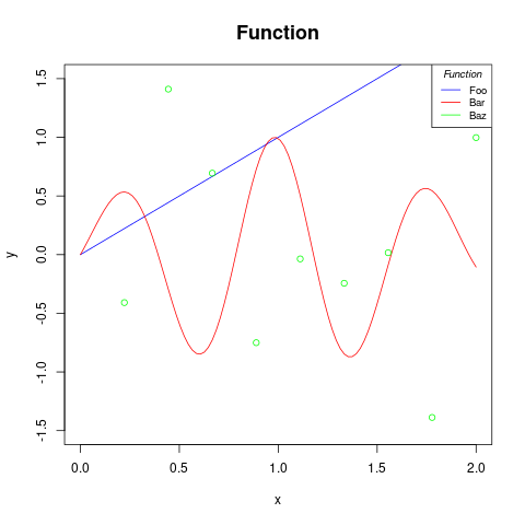
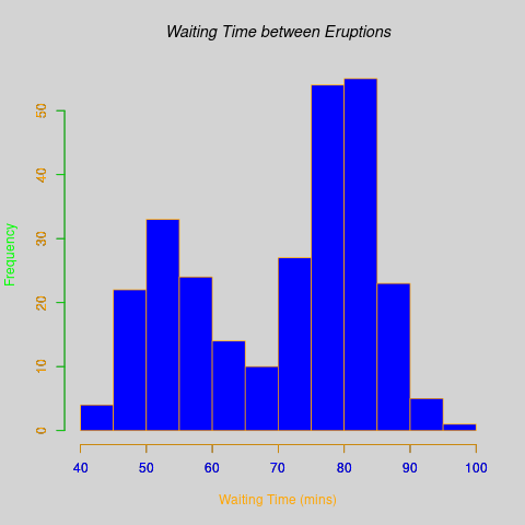
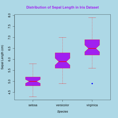
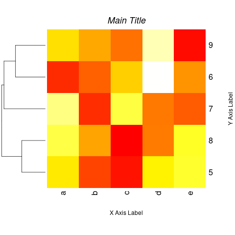

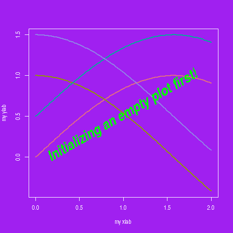


Figure 1
Keywords:
png("fig01.png")

plot(iris[iris$Species == "setosa", ]$Sepal.Length,
     iris[iris$Species == "setosa", ]$Petal.Length,
     col = "red", pch = 1,
     xlab = "Sepal Length", ylab = "Petal Length",
     xlim = range(iris$Sepal.Length), ylim = range(iris$Petal.Length))
points(iris[iris$Species == "versicolor", ]$Sepal.Length,
       iris[iris$Species == "versicolor", ]$Petal.Length,
       col = "green", pch = 2)
points(iris[iris$Species == "virginica", ]$Sepal.Length,
       iris[iris$Species == "virginica", ]$Petal.Length,
       col = "blue", pch = 3)
legend(6.5, 3,
       title = "Species",
       legend = c("Setosa", "Versicolor", "Virginica"),
       col = c("red", "green", "blue"),
       pch = c(1, 2, 3),
       bg = "orange")

dev.off()
Figure 2
Keywords:
png("fig02.png")

x <- seq(0, 2, length.out = 100)
foo <- function(x) x
bar <- function(x) exp(-(x - 1)^2) * sin(x * 8)
points_data <- data.frame(x = seq(0, 2, length = 10), y = rnorm(10))
plot(x, foo(x), type = "l", col = "blue", xlim = c(0, 2), ylim = c(-1.5, 1.5),
     xlab = "x", ylab = "y", main = "Function", cex.main = 1.5)
lines(x, bar(x), col = "red")
points(points_data$x, points_data$y, col = "green")
legend("topright", legend = c("Foo", "Bar", "Baz"), lty = 1, col = c("blue", "red", "green"),
         cex = 0.8, title = expression(bold(italic("Function"))))

dev.off()
Figure 3
Keywords:
png("fig03.png")

data(faithful)

par(bg = "lightgrey")
hist(faithful$waiting,
     main = expression(italic("Waiting Time between Eruptions")),
     breaks = seq(40, 100, by = 5),
     xlab = NULL, ylab = NULL,
     col = "blue", border = "orange", bg = "grey")
axis(side = 1, col.axis = "blue", col = "orange")
title(xlab = "Waiting Time (mins)",
        col.lab = "orange", line = 3)
axis(side = 2, col.axis = "orange", col = "green")
title(ylab = "Frequency",
        col.lab = "green", line = 3)

dev.off()
Figure 4
Keywords:
png("fig04.png")

data(iris)

par(bg = "lightblue", mar = c(5, 4, 4, 2) + 0.1)

boxplot(iris$Sepal.Length ~ iris$Species,
          main = "Distribution of Sepal Length in Iris Dataset",
          col.main = "purple",
          xlab = expression(italic("Species")),
          ylab = "Sepal Length (cm)",
          col = "purple",
          border = "red",
          notch = TRUE,
          boxwex = 0.5,
          staplewex = 0.5,
          outpch = 16,
          outcol = "blue",
          horizontal = FALSE)

dev.off()
Figure 5
Keywords:
png("fig05.png")

nrows <- 5
ncols <- 5
data <- matrix(runif(nrows * ncols), nrow = nrows)
rownames <- as.character(5:9)
colnames <- letters[1:5]

heatmap(data,
          Rowv = TRUE, # include row dendrogram
          Colv = NA,
          xlab = "X Axis Label",
          ylab = "Y Axis Label",
          main = expression(bold(italic("Main Title"))),
          labRow = rownames,
          labCol = colnames,
          col = heat.colors(256))

dev.off()
Figure 6
Keywords: matrix plotting, multiple plotting
png("fig06.png")

n <- 100
x <- seq(0, 2, length.out = n)

y_lines <- matrix(NA, nrow = n, ncol = 2)
y_lines[,1] <- sin(x)
y_lines[,2] <- cos(x)
y_points <- matrix(NA, nrow = n, ncol = 2)
y_points[,1] <- rnorm(n = n, mean = sin(x))
y_points[,2] <- rnorm(n = n, mean = cos(x))

matplot(x, y_lines, type = "l", lwd = 3,
        ylim = c(min(y_points), max(y_points)),
        col = c("red", "blue"),
        ylab = "my ylab", xlab = "my xlab")
matpoints(x, y_points, pch = 1, col = c("red", "blue"))
text(x = 1, y = 0,
     labels = "matplot, matpoints and matlines",
     srt = 30, cex = 2.5, font = 4)

dev.off()
Figure 7
Keywords: matrix plotting, multiple plotting
png("fig07.png")

n <- 100
x <- seq(0, 2, length.out = n)
y_lines <- matrix(NA, nrow = n, ncol = 4)
y_lines[,1] <- sin(x)
y_lines[,2] <- cos(x)
y_lines[,3] <- sin(x) + 0.5
y_lines[,4] <- cos(x) + 0.5

## Play with some of the colours
col_codes <- hcl.colors(n = ncol(y_lines), palette = "Dark 3")
par(bg = "purple",
    fg = "white",
    col.axis = "white",
    col.lab = "white",
    col.main = "white")

## NOTE this initializes an empty plot first.
plot(0, 0,
     type = "n",
     xlim = range(x), ylim = range(y_lines),
     xlab = "my xlab", ylab = "my ylab")
for (jx in seq_len(ncol(y_lines))) {
  lines(x, y_lines[,jx], col = col_codes[jx], lwd = 2)
}
text(x = 1, y = 0.5,
     labels = "Initializing an empty plot first!",
     col = "green",
     srt = 30, cex = 2.5, font = 4)


dev.off()
Figure 8
Keywords: image plot, matrix plotting, colour scale
png("fig08.png")

n <- 20
x <- seq(-pi, pi, length.out = n)
y <- seq(-pi, pi, length.out = n)
mixing_matrix <- outer(x, y,
                       function(x, y) sin(x) * cos(y) + cos(2 * x - y))
tick_at <- seq(1, n, length.out = 10)

image(x = seq_len(n),
      y = seq_len(n),
      z = mixing_matrix,
      axes = FALSE,
      ylab = "Foo", xlab = "Bar",
      col = rainbow(10),
      asp = 1)
axis(1, at = tick_at, labels = LETTERS[1:10])
axis(2, at = tick_at, labels = LETTERS[1:10], las = 1)

dev.off()
Figure 9
Keywords: polygon, shaded region, line plot, transparency
png("fig09.png")

x <- 1:100
y <- sin(x / 10)
se <- 0.2

upper <- y + se
lower <- y - se

plot(x, y,
     type = "n",
     ylim = range(lower, upper),
     xlab = "x", ylab = "sin(x / 10)")
polygon(c(x, rev(x)),
        c(upper, rev(lower)),
        col = "green",
        border = "red")
lines(x, y, lwd = 2, col = "purple")

dev.off()